
1 引言
表 1 系统(1.1)相关变量和参数的意义
| 变量(参数) | 意义 |
| 浮游植物的密度 | |
| 浮游动物的密度 | |
| 浮游植物种内干扰系数 | |
| 成熟捕食者的捕食率 | |
| 反应时间 | |
| 捕食者(浮游动物)之间的干扰程度 | |
| 喂食率 | |
| 转换效率 | |
| 浮游动物的死亡率 | |
| 时滞 | |
| Crowley-Martin[13] 功能反应 |
基于上述讨论, 我们在系统(1.1)引入如下代数方程
其中
初始条件
2 局部稳定性分析
2.1 零收益系统的稳定性分析
当生态经济平衡发生(
解系统(2.1)的第三个方程, 有
把
把
假设
定理2.1 当条件
证 由假设
令
其中
定理2.2 在定理2.1的条件下, 系统(1.2)的生态学平衡点
证 系统(2.2)的特征矩阵是
可得系统(2.2)的特征方程是
接下来, 将利用反证法说明特征值
分离上式的虚部和实部得
注意到
注2.1 定理2.2表明, 当经济效益为零且
2.2 正收益系统的稳定性分析
事实上, 我们更关心的是正经济效益(
成立, 则
其中
令
其中
由此, 得到系统(2.6)的特征方程
其中
首先, 考虑当
定理2.3 若
证 当
其中
令
注意到
然后假设
其中
求解方程(2.9)可得
注意到
假设方程(2.11)至少有一个正实根
进一步定义分岔点
最后, 假设
其中
定理2.4 令
证 对特征方程(2.7)的两边关于
化简可得
因此
假设
定理2.5 假设
3 数值模拟
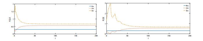
3.1 零经济收益下系统的稳定性
选择系统参数
图 1
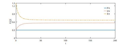
图 2
3.2 正经济收益下系统的稳定性和Hopf分岔
选择参数
图 3
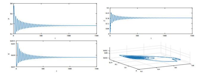
图 3
系统(1.2)的积分曲线和相图.
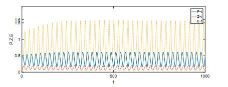
图 4
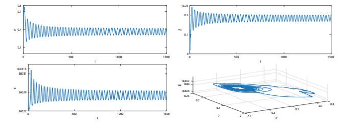
图 4
系统(1.2)的积分曲线和相图.
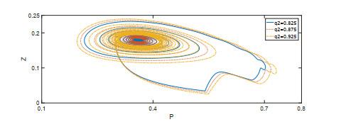
3.3 经济效益对系统的影响
接下来, 考虑经济效益
图 5
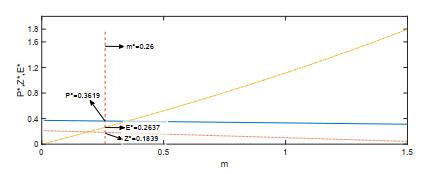
图 6
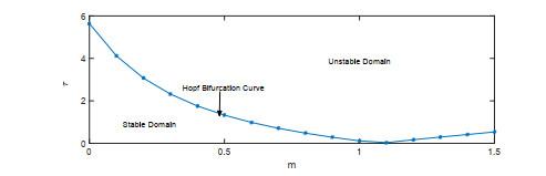
图 7
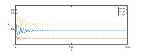
图 8
3.4 分数阶阶数的影响
图 9
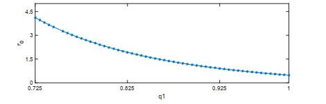
图 10
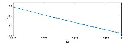
图 11和图 12是
图 11
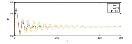
图 12
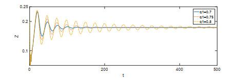
图 13
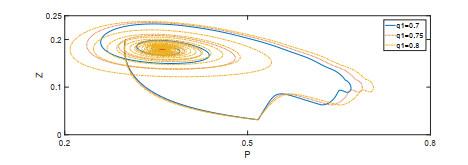
图 14
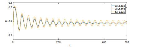
图 15
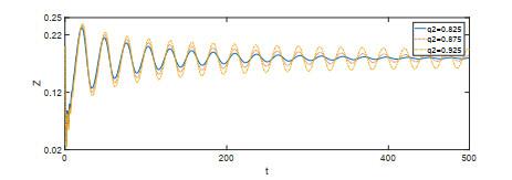
图 16
4 结论
考虑了经济效益的影响, 本文提出了一类时滞的分数阶微分-代数捕食-被捕食系统, 研究了经济效益、分数阶阶数和时滞对此系统稳定性的影响. 所得解结果表明:
(1) 在零经济收益条件下, 系统的正平衡点是局部渐近稳定的; 在正经济收益条件下, 系统的正平衡点附近产生了Hopf分岔;
(2) 分数阶阶数可以抑制所研究系统的振荡;
(3) 时滞是生态系统稳定性改变的原因, 当时滞超过一定阈值时, 系统发生Hopf分岔产生周期解.
E-mail:
参考文献
The significance of microalgal blooms for fisheries and for the export of particulate organic carbon in oceans
DOI:10.1093/plankt/12.4.681 [本文引用: 1]
The dynamics of a harvested predator-prey system with Holling type IV functional response
Dynamic analysis of fractional-order singular Holling type-Ⅱ predator-prey system
Fish and nutrients interplay determines algal biomass: a minimal model
DOI:10.2307/3545491
Qualitative analysis of delayed SIR epidemic model with a saturated incidence rate
DOI:10.1155/2012/408637 [本文引用: 1]
Pattern formation and selection in a diffusive predator-prey system with ratio-dependent functional response
Plankton lattices and the role of chaos in plankton patchiness
Hopf bifurcation in a reaction-diffusive two-spcies model with nonlocal delay effect and general functional response
DOI:10.1016/j.chaos.2016.12.022 [本文引用: 1]
Numerical modelling in biosciences using delay differential equations
Existence of positive periodic solutions of competitor-competitor-mutualist Lotka-Volterra systems with infinite delays
Sensitivity analysis of dynamic systems with time lags
DOI:10.1016/S0377-0427(02)00659-3 [本文引用: 1]
Functional response and interference within and between year classes of a dragonfly population
Hopf bifurcation and spatial patterns of a delayed biological economic system with diffusion
DOI:10.1016/j.amc.2015.05.089 [本文引用: 1]
Solving an inverse heat conduction problem using a non-integer identified model
DOI:10.1016/S0017-9310(00)00310-0 [本文引用: 1]
Optimization of fractional order dynamic chemical processing systems
DOI:10.1021/ie401317r [本文引用: 1]
Equilibrium points, stability and numerical solutions of fractional-order predator-prey and rabies models
DOI:10.1016/j.jmaa.2006.01.087 [本文引用: 1]
A novel strategy of bifurcation control for a delayed fractional predator-prey model
DOI:10.1016/j.amc.2018.11.031 [本文引用: 3]
Hopf bifurcation and chaos in fractional-order modified hybrid optical system
Fractionalization of optical beams: I. Planar analysis
Dynamic analysis of a fractional-order single-species model with diffusion
DOI:10.15388/NA.2017.3.2 [本文引用: 1]
The economic theory of a common property resource: The fishery
Bifurcations of a class of singular biological economic models
DOI:10.1016/j.chaos.2007.09.010 [本文引用: 2]
Bifurcation analysis and control of a differential-algebraic predator-prey model with Allee effect and time delay
Hopf bifurcation and stability for a differential-algebraic biological economic system
DOI:10.1016/j.amc.2010.05.065 [本文引用: 2]
Dynamic analysis of fractional-order predator-prey biological economic system with Holling type Ⅱ functional response
DOI:10.1007/s11071-019-04796-y [本文引用: 1]
Dynamic analysis of fractional-order singular Holling type-Ⅱ predator-prey system
DOI:10.1016/j.amc.2017.05.067 [本文引用: 1]
