1
2004
... 的极限环最大个数及分布如何? 一百多年来, 出现了大量这方面的工作, 但是, 这个问题是非常难的, 即使对于 n = 2 的情形都还没有被完全解决, 仍然是一个公开问题, 这个问题研究进展和部分有效的研究方法可以参见综述性文献[4, 6, 23-24, 27, 32-33]. 基于Hilbert第十六问题的研究难度, Arnold[2]在1977年首次提出弱化形式的Hilbert第十六问题[1, 3], 研究如下系统的Abel积分零点个数, 即系统的Poincaré 分支意义下的极限环个数 ...
Loss of stability of self-oscillations close to resonance and versal deformations of equivariant vector fields
2
1977
... 的极限环最大个数及分布如何? 一百多年来, 出现了大量这方面的工作, 但是, 这个问题是非常难的, 即使对于 n = 2 的情形都还没有被完全解决, 仍然是一个公开问题, 这个问题研究进展和部分有效的研究方法可以参见综述性文献[4, 6, 23-24, 27, 32-33]. 基于Hilbert第十六问题的研究难度, Arnold[2]在1977年首次提出弱化形式的Hilbert第十六问题[1, 3], 研究如下系统的Abel积分零点个数, 即系统的Poincaré 分支意义下的极限环个数 ...
... 事实上, I(h, \delta) 是系统(1.2)后继函数或Poincaré映射的关于 \varepsilon 渐近展开式的一阶近似, I(h, \delta) 的零点的最大个数提供了系统(1.2)的极限环分支的最大个数, 参见文献[2, 11, 15-16, 22]. ...
Ten problems
1
1990
... 的极限环最大个数及分布如何? 一百多年来, 出现了大量这方面的工作, 但是, 这个问题是非常难的, 即使对于 n = 2 的情形都还没有被完全解决, 仍然是一个公开问题, 这个问题研究进展和部分有效的研究方法可以参见综述性文献[4, 6, 23-24, 27, 32-33]. 基于Hilbert第十六问题的研究难度, Arnold[2]在1977年首次提出弱化形式的Hilbert第十六问题[1, 3], 研究如下系统的Abel积分零点个数, 即系统的Poincaré 分支意义下的极限环个数 ...
A unified proof on the weak Hilbert 16th problem for n=2
2
2006
... 的极限环最大个数及分布如何? 一百多年来, 出现了大量这方面的工作, 但是, 这个问题是非常难的, 即使对于 n = 2 的情形都还没有被完全解决, 仍然是一个公开问题, 这个问题研究进展和部分有效的研究方法可以参见综述性文献[4, 6, 23-24, 27, 32-33]. 基于Hilbert第十六问题的研究难度, Arnold[2]在1977年首次提出弱化形式的Hilbert第十六问题[1, 3], 研究如下系统的Abel积分零点个数, 即系统的Poincaré 分支意义下的极限环个数 ...
... 然而, 弱化形式的Hilbert第十六问题依旧难度很大, 目前仅对 n = 2 的情况彻底解决, 见多位学者的系列工作[12, 21, 26, 42], 统一的证明见文献[4]. 学者们关注更加简单的形式的系统(1.2), 具有较强应用背景的多项式Liénard系统 ...
Cyclicity of several quadratic reversible systems with center of genus one
1
2011
... 关于系统(1.1)的Abel积分零点个数上界, 根据不同特点的系统, 学者们提出了辐角原理[23, 31]、直接法[5, 13, 25, 29]、几何方法[7-10, 28]等很多有效的方法. 本文使用Abel积分生成元的Chebyshev系统判定理论来研究Abel积分零点个数上界, 相关的定义详见参考文献[13, 25]. ...
1
2007
... 的极限环最大个数及分布如何? 一百多年来, 出现了大量这方面的工作, 但是, 这个问题是非常难的, 即使对于 n = 2 的情形都还没有被完全解决, 仍然是一个公开问题, 这个问题研究进展和部分有效的研究方法可以参见综述性文献[4, 6, 23-24, 27, 32-33]. 基于Hilbert第十六问题的研究难度, Arnold[2]在1977年首次提出弱化形式的Hilbert第十六问题[1, 3], 研究如下系统的Abel积分零点个数, 即系统的Poincaré 分支意义下的极限环个数 ...
Perturbations from an elliptic Hamiltonian of degree four: (Ⅰ) Saddle loop and two saddle cycle
2
2001
... Dumortier和Li[7-10]系统的研究了不同情况的类型为 (3, 2) 系统(1.4), 得到Abel积分零点个数并得到其上确界及分支图. ...
... 关于系统(1.1)的Abel积分零点个数上界, 根据不同特点的系统, 学者们提出了辐角原理[23, 31]、直接法[5, 13, 25, 29]、几何方法[7-10, 28]等很多有效的方法. 本文使用Abel积分生成元的Chebyshev系统判定理论来研究Abel积分零点个数上界, 相关的定义详见参考文献[13, 25]. ...
Perturbations from an elliptic Hamiltonian of degree four: (Ⅱ) Cuspidal loop
0
2001
Perturbation from an elliptic Hamiltonian of degree four: Ⅲ Global center
0
2003
Perturbations from an elliptic Hamiltonian of degree four: (Ⅳ) Figure eight-loop
2
2003
... Dumortier和Li[7-10]系统的研究了不同情况的类型为 (3, 2) 系统(1.4), 得到Abel积分零点个数并得到其上确界及分支图. ...
... 关于系统(1.1)的Abel积分零点个数上界, 根据不同特点的系统, 学者们提出了辐角原理[23, 31]、直接法[5, 13, 25, 29]、几何方法[7-10, 28]等很多有效的方法. 本文使用Abel积分生成元的Chebyshev系统判定理论来研究Abel积分零点个数上界, 相关的定义详见参考文献[13, 25]. ...
1
1992
... 事实上, I(h, \delta) 是系统(1.2)后继函数或Poincaré映射的关于 \varepsilon 渐近展开式的一阶近似, I(h, \delta) 的零点的最大个数提供了系统(1.2)的极限环分支的最大个数, 参见文献[2, 11, 15-16, 22]. ...
The infinitesimal 16th Hilbert problem in the quadratic case
1
2001
... 然而, 弱化形式的Hilbert第十六问题依旧难度很大, 目前仅对 n = 2 的情况彻底解决, 见多位学者的系列工作[12, 21, 26, 42], 统一的证明见文献[4]. 学者们关注更加简单的形式的系统(1.2), 具有较强应用背景的多项式Liénard系统 ...
A Chebyshev criterion for Abelian integrals
4
2011
... 关于系统(1.1)的Abel积分零点个数上界, 根据不同特点的系统, 学者们提出了辐角原理[23, 31]、直接法[5, 13, 25, 29]、几何方法[7-10, 28]等很多有效的方法. 本文使用Abel积分生成元的Chebyshev系统判定理论来研究Abel积分零点个数上界, 相关的定义详见参考文献[13, 25]. ...
... 等很多有效的方法. 本文使用Abel积分生成元的Chebyshev系统判定理论来研究Abel积分零点个数上界, 相关的定义详见参考文献[13, 25]. ...
... 在研究一些系统时, s 的值不能满足条件(ⅲ), 引理2.1并不能直接应用, 此时可以使用如下引理2.2, 提高 I_i(h) 中 y 的次数, 克服上述困难, 参见文献[13]中的引理4.1. ...
... Abel积分零点个数的Chebyshev性质的代数判定方法最初的思想是来源于文献[25], 后来在文献[13]和文献[30]中得以推广和发展. ...
Asymptotic expansions of Melnikov functions and limit cycle bifurcations
1
2012
... 计算Abel积分零点个数的一个有效的方法是研究(1.2) 周期环域 \{L_{h}\} 端点附近的渐近展开式(参见文献[14, 37]及[38]). 假如系统(1.2)的周期环域的内边界是初等中心 C(0, 0) 满足 {H}(C) = 0 , 外边界是连接双曲鞍点 S_1(x_1, y_1) 的同宿环 L_{h_s} , 满足 {H}(x_1, y_1) = h_s , 那么 ...
Existence of at most 1, 2, or 3 zeros of a melnikov function and limit cycles
1
2001
... 事实上, I(h, \delta) 是系统(1.2)后继函数或Poincaré映射的关于 \varepsilon 渐近展开式的一阶近似, I(h, \delta) 的零点的最大个数提供了系统(1.2)的极限环分支的最大个数, 参见文献[2, 11, 15-16, 22]. ...
On Hopf cyclicity of planar systems
1
2000
... 事实上, I(h, \delta) 是系统(1.2)后继函数或Poincaré映射的关于 \varepsilon 渐近展开式的一阶近似, I(h, \delta) 的零点的最大个数提供了系统(1.2)的极限环分支的最大个数, 参见文献[2, 11, 15-16, 22]. ...
Limit cycles by Hopf and homoclinic bifurcations for near-Hamiltonian systems
1
2007
... 注2.1 引理2.5是文献[17]的转述, 较为清晰的证明见文献[36]. ...
Limit cycles near homoclinic and heteroclinic loops
1
2008
... 引理2.4[18-19] 假设 (x, y) 在双曲鞍点 S_1(x_1, y_1) 附近 ...
Hopf bifurcations for near-Hamiltonian systems
3
2009
... 引理2.3[19] 假设 (x, y) 在初等中心 C(0, 0) 附近 ...
... 引理2.4[18-19] 假设 (x, y) 在双曲鞍点 S_1(x_1, y_1) 附近 ...
... 那么系统的Hamiltonian函数就变为(2.3) 式的形式, 而积分 I(h, \delta) 保持不变. 对系统(4.1) 应用文献[19]中的计算方法得 ...
Mathematical problems
1
1902
... 德国数学家Hilbert在1900年世界数学家大会上提出了23个著名的数学问题[20], 其中, 第十六个问题的第二部分是: 平面实 n 次多项式自治系统 ...
On the number of limit cycles in perturbations of quadratic Hamiltonian systems
1
1994
... 然而, 弱化形式的Hilbert第十六问题依旧难度很大, 目前仅对 n = 2 的情况彻底解决, 见多位学者的系列工作[12, 21, 26, 42], 统一的证明见文献[4]. 学者们关注更加简单的形式的系统(1.2), 具有较强应用背景的多项式Liénard系统 ...
1
1991
... 事实上, I(h, \delta) 是系统(1.2)后继函数或Poincaré映射的关于 \varepsilon 渐近展开式的一阶近似, I(h, \delta) 的零点的最大个数提供了系统(1.2)的极限环分支的最大个数, 参见文献[2, 11, 15-16, 22]. ...
Abelian integrals and limit cycles
2
2012
... 的极限环最大个数及分布如何? 一百多年来, 出现了大量这方面的工作, 但是, 这个问题是非常难的, 即使对于 n = 2 的情形都还没有被完全解决, 仍然是一个公开问题, 这个问题研究进展和部分有效的研究方法可以参见综述性文献[4, 6, 23-24, 27, 32-33]. 基于Hilbert第十六问题的研究难度, Arnold[2]在1977年首次提出弱化形式的Hilbert第十六问题[1, 3], 研究如下系统的Abel积分零点个数, 即系统的Poincaré 分支意义下的极限环个数 ...
... 关于系统(1.1)的Abel积分零点个数上界, 根据不同特点的系统, 学者们提出了辐角原理[23, 31]、直接法[5, 13, 25, 29]、几何方法[7-10, 28]等很多有效的方法. 本文使用Abel积分生成元的Chebyshev系统判定理论来研究Abel积分零点个数上界, 相关的定义详见参考文献[13, 25]. ...
弱化希尔伯特第16问题及其研究现状
1
2010
... 的极限环最大个数及分布如何? 一百多年来, 出现了大量这方面的工作, 但是, 这个问题是非常难的, 即使对于 n = 2 的情形都还没有被完全解决, 仍然是一个公开问题, 这个问题研究进展和部分有效的研究方法可以参见综述性文献[4, 6, 23-24, 27, 32-33]. 基于Hilbert第十六问题的研究难度, Arnold[2]在1977年首次提出弱化形式的Hilbert第十六问题[1, 3], 研究如下系统的Abel积分零点个数, 即系统的Poincaré 分支意义下的极限环个数 ...
弱化希尔伯特第16问题及其研究现状
1
2010
... 的极限环最大个数及分布如何? 一百多年来, 出现了大量这方面的工作, 但是, 这个问题是非常难的, 即使对于 n = 2 的情形都还没有被完全解决, 仍然是一个公开问题, 这个问题研究进展和部分有效的研究方法可以参见综述性文献[4, 6, 23-24, 27, 32-33]. 基于Hilbert第十六问题的研究难度, Arnold[2]在1977年首次提出弱化形式的Hilbert第十六问题[1, 3], 研究如下系统的Abel积分零点个数, 即系统的Poincaré 分支意义下的极限环个数 ...
A criterion for determining the monotonicity of the ratio of two abelian integrals
3
1996
... 关于系统(1.1)的Abel积分零点个数上界, 根据不同特点的系统, 学者们提出了辐角原理[23, 31]、直接法[5, 13, 25, 29]、几何方法[7-10, 28]等很多有效的方法. 本文使用Abel积分生成元的Chebyshev系统判定理论来研究Abel积分零点个数上界, 相关的定义详见参考文献[13, 25]. ...
... , 25]. ...
... Abel积分零点个数的Chebyshev性质的代数判定方法最初的思想是来源于文献[25], 后来在文献[13]和文献[30]中得以推广和发展. ...
Remarks on 16th weak Hilbert problem for n = 2
1
2002
... 然而, 弱化形式的Hilbert第十六问题依旧难度很大, 目前仅对 n = 2 的情况彻底解决, 见多位学者的系列工作[12, 21, 26, 42], 统一的证明见文献[4]. 学者们关注更加简单的形式的系统(1.2), 具有较强应用背景的多项式Liénard系统 ...
Hilberts 16th problem and bifurcations of planar polynomial vector fields
1
2003
... 的极限环最大个数及分布如何? 一百多年来, 出现了大量这方面的工作, 但是, 这个问题是非常难的, 即使对于 n = 2 的情形都还没有被完全解决, 仍然是一个公开问题, 这个问题研究进展和部分有效的研究方法可以参见综述性文献[4, 6, 23-24, 27, 32-33]. 基于Hilbert第十六问题的研究难度, Arnold[2]在1977年首次提出弱化形式的Hilbert第十六问题[1, 3], 研究如下系统的Abel积分零点个数, 即系统的Poincaré 分支意义下的极限环个数 ...
The cyclicity of period annuli of a class of quadratic reversible systems with two centers
1
2012
... 关于系统(1.1)的Abel积分零点个数上界, 根据不同特点的系统, 学者们提出了辐角原理[23, 31]、直接法[5, 13, 25, 29]、几何方法[7-10, 28]等很多有效的方法. 本文使用Abel积分生成元的Chebyshev系统判定理论来研究Abel积分零点个数上界, 相关的定义详见参考文献[13, 25]. ...
The monotonicity of the ratio of two Abelian integrals
1
2013
... 关于系统(1.1)的Abel积分零点个数上界, 根据不同特点的系统, 学者们提出了辐角原理[23, 31]、直接法[5, 13, 25, 29]、几何方法[7-10, 28]等很多有效的方法. 本文使用Abel积分生成元的Chebyshev系统判定理论来研究Abel积分零点个数上界, 相关的定义详见参考文献[13, 25]. ...
Bounding the number of zeros of certain Abelian integrals
2
2011
... 关于其线性组合的零点个数有如下结果(见文献[30]). ...
... Abel积分零点个数的Chebyshev性质的代数判定方法最初的思想是来源于文献[25], 后来在文献[13]和文献[30]中得以推广和发展. ...
Number of zeros of complete elliptic integrals
1
1984
... 关于系统(1.1)的Abel积分零点个数上界, 根据不同特点的系统, 学者们提出了辐角原理[23, 31]、直接法[5, 13, 25, 29]、几何方法[7-10, 28]等很多有效的方法. 本文使用Abel积分生成元的Chebyshev系统判定理论来研究Abel积分零点个数上界, 相关的定义详见参考文献[13, 25]. ...
On dynamical systems close to hamiltonian ones
1
1934
... 的极限环最大个数及分布如何? 一百多年来, 出现了大量这方面的工作, 但是, 这个问题是非常难的, 即使对于 n = 2 的情形都还没有被完全解决, 仍然是一个公开问题, 这个问题研究进展和部分有效的研究方法可以参见综述性文献[4, 6, 23-24, 27, 32-33]. 基于Hilbert第十六问题的研究难度, Arnold[2]在1977年首次提出弱化形式的Hilbert第十六问题[1, 3], 研究如下系统的Abel积分零点个数, 即系统的Poincaré 分支意义下的极限环个数 ...
Mathematical problems for the next century
1
1998
... 的极限环最大个数及分布如何? 一百多年来, 出现了大量这方面的工作, 但是, 这个问题是非常难的, 即使对于 n = 2 的情形都还没有被完全解决, 仍然是一个公开问题, 这个问题研究进展和部分有效的研究方法可以参见综述性文献[4, 6, 23-24, 27, 32-33]. 基于Hilbert第十六问题的研究难度, Arnold[2]在1977年首次提出弱化形式的Hilbert第十六问题[1, 3], 研究如下系统的Abel积分零点个数, 即系统的Poincaré 分支意义下的极限环个数 ...
Bounding the number of limit cycles for a polynomial Liénard system by using regular chains
1
2017
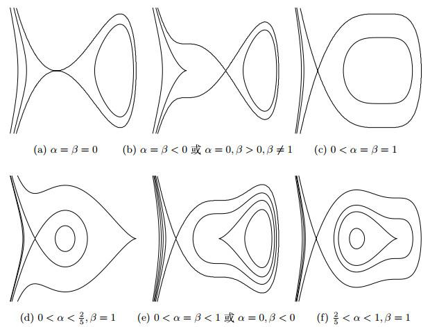
... 当 \alpha = \beta = 1 时, 系统 (1.5)_{\varepsilon = 0} 周期环域内外边界分别是幂零中心和连接双曲鞍点的同宿轨, 如图 1(c). 孙, 苏和韩[35]以及王[39]分别研究了此情况的Abel积分零点个数, 得到其上界是5或6和下界是3. 孙和黄[34]证明了另一类此情况的Abel积分零点个数上界是6和下界是4. ...
On the number of zeros of Abelian integral for some Liénard system of type (4, 3)
1
2013
... 当 \alpha = \beta = 1 时, 系统 (1.5)_{\varepsilon = 0} 周期环域内外边界分别是幂零中心和连接双曲鞍点的同宿轨, 如图 1(c). 孙, 苏和韩[35]以及王[39]分别研究了此情况的Abel积分零点个数, 得到其上界是5或6和下界是3. 孙和黄[34]证明了另一类此情况的Abel积分零点个数上界是6和下界是4. ...
一类扰动超椭圆Hamilton系统的Abel积分零点个数上确界
2
2015
... 当 \alpha = \beta<0 或者 \alpha = 0, \beta>0 , \beta\neq 1 时, 系统 (1.5)_{\varepsilon = 0} 周期环域内边界是初等中心外边界是连接双曲鞍点的同宿轨, 环域外部是幂零尖点, 如图 1(b). 孙和吴[36]研究了当 \alpha = \beta = -3 时的特殊情况, 得到其Abel积分零点个数上确界. 对于一般的 \alpha = \beta<0 未见相关结果. ...
... 注2.1 引理2.5是文献[17]的转述, 较为清晰的证明见文献[36]. ...
Bifurcation of limit cycles in small perturbation of a class of Liénard systems
2
2014
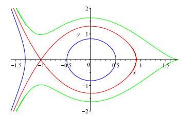
... 计算Abel积分零点个数的一个有效的方法是研究(1.2) 周期环域 \{L_{h}\} 端点附近的渐近展开式(参见文献[14, 37]及[38]). 假如系统(1.2)的周期环域的内边界是初等中心 C(0, 0) 满足 {H}(C) = 0 , 外边界是连接双曲鞍点 S_1(x_1, y_1) 的同宿环 L_{h_s} , 满足 {H}(x_1, y_1) = h_s , 那么 ...
... (ⅱ) 为了探讨 q(x, z) 和 p_2(x, z) 是否有满足条件的公共根, 我们把 q(x, z) 和 p_2(x, z) 代入到文献[37]中的附录A的程序中 ...
Hopf and homoclinic bifurcations for near-Hamiltonian systems
1
2017
... 计算Abel积分零点个数的一个有效的方法是研究(1.2) 周期环域 \{L_{h}\} 端点附近的渐近展开式(参见文献[14, 37]及[38]). 假如系统(1.2)的周期环域的内边界是初等中心 C(0, 0) 满足 {H}(C) = 0 , 外边界是连接双曲鞍点 S_1(x_1, y_1) 的同宿环 L_{h_s} , 满足 {H}(x_1, y_1) = h_s , 那么 ...
Estimate of the number of zeros of Abelian integrals for a perturbation of hyperelliptic Hamiltonian system with nilpotent center
1
2012
... 当 \alpha = \beta = 1 时, 系统 (1.5)_{\varepsilon = 0} 周期环域内外边界分别是幂零中心和连接双曲鞍点的同宿轨, 如图 1(c). 孙, 苏和韩[35]以及王[39]分别研究了此情况的Abel积分零点个数, 得到其上界是5或6和下界是3. 孙和黄[34]证明了另一类此情况的Abel积分零点个数上界是6和下界是4. ...
On the number of limit cycles in small perturbations of a class of hyperelliptic Hamiltonian systems with one nilpotent saddle
1
2011
... 当 \alpha = \beta = 0 时, 系统 (1.5)_{\varepsilon = 0} 周期环域边界分别是初等中心和连接幂零鞍点的同宿轨, 见图 1(a). 王和肖[40]证明了此情况的Abel积分零点个数上界是4和下界是3. ...
Bifurcations on a five-parameter family of planar vector field
1
2008
... 其中 \alpha 和 \beta 是实参数. 根据参数的不同取值, 系统 (1.5)_{\varepsilon = 0} 具有6种不同情况的周期环域相图[41], 见图 1. ...
On the number of limit cycles of a class of quadratic Hamiltonian systems under quadratic perturbations
1
1997
... 然而, 弱化形式的Hilbert第十六问题依旧难度很大, 目前仅对 n = 2 的情况彻底解决, 见多位学者的系列工作[12, 21, 26, 42], 统一的证明见文献[4]. 学者们关注更加简单的形式的系统(1.2), 具有较强应用背景的多项式Liénard系统 ...


