

1 引言
时滞现象在生物神经网络与人工神经网络中广泛存在, 它是导致系统振动与不稳定性的关键因素之一. 因此, 针对具有时滞特性的神经网络进行深入研究一直是该领域的热点话题[1,2]. 比例时滞是一种无界时滞, 文献 [3] 基于 QoS 路由决策需要比例时滞保证且可由神经网络实现提出了比例时滞神经网络, 此后比例时滞神经网络的动力学得到了国内外学者的广泛研究, 如稳定性[4,5,6,7]、无源性[8]、周期性[9]等. 同步性作为稳定性的延申, 由于其在保密通信[10]、图像保护[11]等领域的应用而得到了广泛研究, 如文献 [12] 利用比较原理和时间尺度理论探讨了一类时标型非自治比例时滞神经网络的同步问题.文献 [13] 通过设计量化控制技术, 利用 Wirdinger 不等式及构造 Lyapunov -Krasovskii 泛函分析了比例时滞耦合反应扩散神经网络的渐近同步. 文献 [14] 通过构造 Lyapunov 泛函, 设计合适的控制输入研究了比例时滞递归神经网络的指数同步和多项式同步, 并揭示了指数同步和多项式同步之间的关系.
自从 Babcock 和 Wheeler 在文献 [15] 中提出了惯性神经网络以来, 其动力学研究取得了许多成果[16,17]. 时滞惯性神经网络的同步与混沌控制是近几十年来的研究热点之一[18], 比例时滞惯性神经网络的同步研究也取得一些成果, 如文献 [19] 采用非降阶方法和 Lyapunov 稳定性理论探究了比例时滞的脉冲复值惯性神经网络的全局指数镇定和指数滞后同步. 文献 [20] 利用微分包含理论和降阶变换、设计反馈控制器与自适应控制器以及构造 Lyapunov 泛函探讨了比例时滞惯性忆阻 Cohen-Grossberg 神经网络的全局渐近同步. 文献 [21] 设计反馈控制器、采用降阶方法和构造范数形式的比例时滞微分不等式研究了比例时滞惯性神经网络的全局多项式同步, 但相比其他有界时变时滞惯性神经网络的同步控制研究, 该领域仍有巨大的研究空间.
除了时滞影响, 环境噪声也是系统运行过程中不可避免的因素, 在神经网络中考虑噪声的影响能更好的刻画网络的实际状态, 因此, 随机神经网络的动力学研究具有重要的现实意义.近年来, 对于有界时变时滞的随机神经网络动力学的研究成果较为丰富[22,23,24].然而, 关于比例时滞随机神经网络的动力学研究仍非常有限[25,26], 文献[25] 利用 Lyapunov -Krasovskii 泛函、随机分析理论和 Itô 公式研究了多比例时滞随机递归神经网络状态稳定性的均方指数输入状态稳定性. 文献 [26] 设计了一种延迟反馈控制器和采用 Lyapunov 方法分析了比例时滞随机复值忆阻模糊细胞神经网络的固定时间同步. 目前, 关于比例时滞惯性随机神经网络的均方指数同步研究鲜有报道.
基于这些启发, 本文将考虑一类比例时滞惯性随机神经网络均方指数同控制问题, 并进一步将所研究的均方指数同步应用于图像加密. 本文的创新性及主要贡献总结如下
2 模型描述与预备知识
符号说明:
考虑如下一类比例时滞惯性随机神经网络
其中
将系统 (2.1) 作为驱动系统, 取响应系统如下
其中
作系统 (2.1) 和 (2.2) 的误差系统, 令
其中
其中
本文对
(H
(H
在文献 [27] 中, 对于系统
其中
对于
这里
若
引理 2.1[27] 设
则
定义 2.1 在某一控制器
则称系统 (2.1) 和 (2.2) 能达到均方指数同步.
3 主要结果
设计如下控制器
定理3.1 假设 (H
则系统 (2.1) 和 (2.2) 能达到均方指数同步.
证 令
且
由 (2.4), (2.5) 和 (3.2) 式, 得
由 (H
其中
另一方面, 由 (2.6) 式, 知
这里
由 (3.2)-(3.5) 式, 得
对 (3.6) 式两边取数学期望, 得
其中
由引理 2.1, 由 (3.7) 式, 得
因此, 根据定义 2.1 可知系统 (2.1) 和 (2.2) 在控制器(3.1) 作用下均方指数同步.
注 3.1 本文构造正定的 Lyapunov 泛函 (3.2) 的新颖性有两点: 1) 积分项前面乘上
定理 3.1 是通过构造 Lyapunov 泛函, 结合已知条件等进行系统 (1) 和 (2) 的均方指数同步探究的.接下来, 本文不构造 Lyapunov 泛函, 而是直接通过微积分的相应性质进行均方指数同步分析.
定理 3.2 假设 (H
则系统 (2.1) 和 (2.2) 能达到均方指数同步.
证 由 (2.4) 式, 得
对上式两边从
再由均值不等式, 得
由于
将 (3.10) 式代入 (3.9) 式, 可得
其中
其中
由引理 1 和 (3.12), 可得
即系统 (2.1) 和 (2.2) 在控制器 (3.1) 作用下均方指数同步.
注 3.2 定理 3.1 和 3.2 都依赖于比例时滞因子, 但定理 3.2 不要求
注 3.3 在系统 (2.1) 和 (2.2) 中, 若不考虑随机项, 本文所得结果仍然成立. 当
4 数值算例及图像加密
例 4.1 在系统 (2.1) 和 (2.2) 中, 选取系统参数及控制器参数如下:
此时, 函数
情况 1 存在比例时滞情况下, 取
满足定理 3.1, 因此, 系统 (2.1) 和 (2.2) 在控制器 (3.1) 的作用下能达到均方指数同步.
取初值
图1

图1
(a) 驱动系统 (2.1) 的相图; (b) 不加控制器时响应系统 (2.2) 的相图; (c) 响应系统 (2.2) 在控制器 (3.1) 下的相图
图2

图2
(a) 驱动系统 (2.1) 的状态轨迹; (b) 不加控制器响应系统 (2.2) 的状态轨迹; (c) 响应系统 (2.2) 在控制器 (3.1) 下的状态轨迹
图3

图3
(a) 系统 (2.1) 和 (2.2) 在控制器 (3.1) 下的误差系统的状态轨迹; (b) 无时滞时, 系统 (2.1) 和 (2.2) 在控制器 (3.1) 下的误差系统的状态轨迹.
情况 2 无比例时滞情况下, 此时
满足注 3.3, 因此此时无时滞系统 (2.1) 和 (2.2) 在控制器 (3.1) 的作用下能达到均方指数同步, 如图 3(b) 所示.
例 4.2 以图像的加密和解密为例给出本文所研究的指数同步在保密通信中的应用.
利用例 4.1 中系统 (2.1) 和 (2.2) 的指数同步结果进行图像的加密和解密, 并通过直方图、信息熵、同步误差和散点图等给出其相应的安全性分析.
选取图像
图4

图4
(a) 图像
(1) 像素读取, 读取要进行加密的彩色图像
(2) 置换加密, 生成两组伪随机序列
(3) 图像加密, 基于例 4.1 给出的模型参数和初值, 可以得到驱动系统序列
将矩阵
(4) 图像解密, 由响应系统可得序列
实验结果如图 4(a)-(c) 所示. 图 4(b) 是使用驱动系统序列导出的加密图像, 其掩盖了原始图像中包含的信息. 另一方面, 图 4(c) 是利用响应系统序列重建的解密图像, 从该图可观察到加密图像已完全恢复. 接下来, 将进一步分析所提出的图像加密算法的安全性.
图像信息熵是衡量图像随机性或不确定性水平的关键指标, 定义为

本文通过分析系统在受到不同程度的同步误差时的解密性能, 来检查加密密钥的敏感性. 图5(a)-(c) 出示了图像的解密效果随着同步误差的增加而降低, 表明我们的图像加密算法具有较高的灵敏度. 若将驱动响应系统的混沌序列应用于图像保护, 本文应该努力使同步误差尽可能小
图5

在相邻像素之间, 为了防止统计攻击, 必须减少信息相关性. 表2详细说明了图像中三个不同方向上相邻像素点的相关性, 实验结果表明, 水平、垂直和对角线加密的

图6
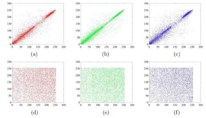
图6
(a) 原图水平相邻像素相关散点图; (b) 原图垂直相邻像素相关散点图; (c) 原图对角相邻像素相关散点图; (d) 加密图像水平散点图; (e) 加密图像垂直散点图; (f) 加密图像对角散点图.
5 结论
本文探究了一类比例时滞惯性随机神经网络的均方指数同步及其在图像加密和解密中的应用. 通过设计反馈控制器, 运用 Itô 公式, 构建 Lyapunov 泛函和利用微积分的性质, 得到了所研究系统均方指数同步的时滞所依赖的代数形式的充分条件, 条件简单, 易于验证. 通过数值例题及仿真验证了所得到理论结果是正确的. 同时, 将例 4.1 中驱动-响应系统的均方指数同步应用于图像的加密和解密, 并从直方图、信息熵、误差比较和散点图的实验结果表明本文设计的同步方案和加密算法对保密通信是合理有效的. 本文的研究方法也适用于比例时滞神经网络的周期性和无源性的研究, 图像加密和解密的方法也可应用于其他神经网络在保密通信中应用.
参考文献
具有混合变时滞的脉冲 Cohen-Grossberg 神经网络的指数同步
Exponential synchronization for impulsive Cohen-Grossberg neural networks with mixed time-varying delays
Intermittent quasi-synchronization criteria of chaotic delayed neural networks with parameter mismatches and stochastic perturbation mismatches via Razumikhin-type approach
On the global dissipativity of a class of cellular neural networks with multi-pantograph delays
基于 Gronwall 积分不等式的比例时滞神经网络稳定性分析
Stability analysis for a class neural network with proportional delay based on the Gronwall integral inequality
Fixed-time stabilization of fuzzy neutral-type inertial neural networks with proportional delays
Fixed-time stabilization of discontinuous neutral neural networks with proportional delays via new fixed-time stability lemmas
Global exponential stability and synchronization for a novel complex-valued neural networks with proportional delays and inhibitory factors
Delay-dependent passivity of impulsive coupled reaction-diffusion neural networks with multi-proportional delays
Global polynomial periodicity and polynomial stability of Cohen-Grossberg neural networks with proportional delays
Finite-time and fixed-time synchronization of a class of inertial neural networks with multi-proportional delays and its application to secure communication
DOI:10.1016/j.neucom.2018.11.020
[本文引用: 1]

Proportional delay, which is different from time-varying delays and distributed delay, is a kind of unbounded delay. The proportional delay system as an important mathematical model often rises in some various fields such as control theory, physics and biology systems. This paper is concerned with the finite-time and the fixed-time synchronization problem for a class of inertial neural networks with multi-proportional delays. First, by constructing a proper variable substitution, the original inertial neural networks with multi-proportional delays can be rewritten as a first-order differential system. Second, by constructing Lyapunov functionals and by using analytical techniques, and together with novel control algorithms, some new and effective criteria are established to achieve finite-time and fixed-time synchronization of the master/slave of addressed systems. Finally, several examples and their simulations are given to illustrate the effectiveness of the proposed method. Furthermore, a secure communication synchronization problem is presented to illustrate the effectiveness of the obtained results. (C) 2018 Published by Elsevier B.V.
Stabilization of nonautonomous recurrent neural networks with bounded and unbounded delays on time scales
DOI:10.1109/TCYB.2019.2922207
PMID:31265426
[本文引用: 1]
A class of nonautonomous recurrent neural networks (NRNNs) with time-varying delays is considered on time scales. Bounded delays and unbounded delays have been taken into consideration, respectively. First, a new generalized Halanay inequality on time scales is constructed by time-scale theory and some analytical techniques. Based on this inequality, the stabilization of NRNNs with bounded delays is discussed on time scales. The results are also applied to the synchronization of a class of drive-response NRNNs. Furthermore, the stabilization of NRNNs with unbounded delays is investigated. Especially, the stabilization of NRNNs with proportional delays is obtained without any variable transformation. The obtained generalized Halanay inequality on time scales develops and extends some existing ones in the literature. The stabilization criteria for the NRNNs with bounded or unbounded delays cover the results of continuous-time and discrete-time NRNNs and hold the results for the systems that involved on time interval as well. Some examples are given to demonstrate the validity of the results. An application to image encryption and decryption is addressed.
Synchronization of timescale-type nonautonomous neural networks with proportional delays
Synchronization of coupled Markovian reaction-diffusion neural networks with proportional delays via quantized control
DOI:10.1109/TNNLS.2018.2853650
PMID:30072345
[本文引用: 2]
The asymptotic synchronization of coupled reaction-diffusion neural networks with proportional delay and Markovian switching topologies is considered in this brief where the diffusion space does not need to contain the origin. The main objectives of this brief are to save communication resources and to reduce the conservativeness of the obtained synchronization criteria, which are carried out from the following two aspects: 1) mode-dependent quantized control technique is designed to reduce control cost and save communication channels and 2) Wirtinger inequality is utilized to deal with the reaction-diffusion terms in a matrix form and reciprocally convex technique combined with new Lyapunov-Krasovskii functional is used to derive delay-dependent synchronization criteria. The obtained results are general and formulated by linear matrix inequalities. Moreover, combined with an optimal algorithm, control gains with the least magnitude are designed.
Exponential synchronization and polynomial synchronization of recurrent neural networks with and without proportional delays
Stability and dynamics of simple electronic neural networks with added inertia
Novel finite-time reliable control design for memristor-based inertial neural networks with mixed time-varying delays
Fixed time stability of nonlinear impulsive systems and its application to inertial neural networks
Sampled-data control for exponential synchronization of delayed inertial neural networks with aperiodic sampling and state quantization
Stabilization and lag synchronization of proportional delayed impulsive complex-valued inertial neural networks
Global asymptotic synchronization of inertial memristive Cohen-Grossberg neural networks with proportional delays
Global polynomial synchronization of proportional delayed inertial neural networks
Finite-time synchronization of chaotic neural networks with mixed time-varying delays and stochastic disturbance
Predefined-time synchronization of stochastic memristor-based bidirectional associative memory neural networks with time-varying delays
基于 LMI 方法的多时滞随机神经网络的指数稳定性
Exponential stability for stochastic neural networks with multiple delays: an LMI approach
Mean-square exponential input-to-state stability of stochastic recurrent neural networks with multi-proportional delays
Fixed-time synchronization of stochastic complex-valued fuzzy neural networks with memristor and proportional delays
