一类具有非等熵 Dusty 气体的两相流模型 Riemann 解的压力消失极限

一类具有非等熵 Dusty 气体的两相流模型 Riemann 解的压力消失极限

金岱广, 何劭弘^,, 吴雨嫣, 蒋伟峰^,^*

中国计量大学理学院杭州 310018

The Vanishing Pressure Limit of Riemann Solutions for a Class of Two-Phase Flow Models with Non-Isentropic Dusty Gases

Jin Daiguang, He Shaohong^,, Wu Yuyan, Jiang Weifeng^,^*

Faculty of Science, China Jiliang University, Hangzhou 310018

通讯作者: * 蒋伟峰，E-mail: casujiang89@cjlu.edu.cn

收稿日期: 2024-11-5 修回日期: 2025-01-26

基金资助:

国家自然科学基金(1240012056)

Received: 2024-11-5 Revised: 2025-01-26

Fund supported:

NSFC(1240012056)

作者简介 About authors

E-mail:s22080701004@cjlu.edu.cn

摘要

该文研究一类具有非等熵 Dusty 气体的两相流模型 Riemann 解在压力消失时的极限行为. 首先, 针对该模型的黎曼问题, 利用特征分析法得到基本波的表达式并在 $(p, u, s)$ 坐标系中构造了黎曼熵解. 然后, 证明了在压力消失时该模型的黎曼解收敛于带相同初值的一维常压力流体模型的黎曼解. 最后, 对该模型的黎曼解在压力消失过程中 $\delta$ -激波和真空状态的形成进行数值模拟, 验证了上述理论分析的结果.

关键词： 非等熵; 两相流模型; 压力消失极限; 黎曼解; $\delta$ -激波; 真空状态

Abstract

This paper studies the cavitation and concentration phenomena of the Riemann solutions for a reduced two-phase mixtures model with non-isentropic dusty gas state as the pressure vanishes. Firstly, we construct the Riemann entropy solutions by characteristic analysis method in $(p, u, s)$ coordinate system. Secondly, we conclude that, the pressureless limit of Riemann solutions for the reduced two-phase mixtures model is just the Riemann solutions for the reduced 2-dimensional pressureless gas dynamics model. Finally, we present numerical simulations which are consistent with our theoretical analysis.

Keywords： non-isentropic; two-phase mixtures model; pressureless limit; Riemann problem; Delta shock wave; vacuum state

PDF (735KB) 元数据多维度评价相关文章导出 EndNote| Ris| Bibtex 收藏本文

本文引用格式

金岱广, 何劭弘, 吴雨嫣, 蒋伟峰. 一类具有非等熵 Dusty 气体的两相流模型 Riemann 解的压力消失极限[J]. 数学物理学报, 2025, 45(2): 371-388

Jin Daiguang, He Shaohong, Wu Yuyan, Jiang Weifeng. The Vanishing Pressure Limit of Riemann Solutions for a Class of Two-Phase Flow Models with Non-Isentropic Dusty Gases[J]. Acta Mathematica Scientia, 2025, 45(2): 371-388

1 引言

考虑简化的非等熵两相流模型^[1]

$\begin{cases}\rho_{t}+(\rho u)_{x}=0, \\(\rho u)_{t}+(\rho u^{2}+p(\rho, s))_{x}=0, \\(\rho s)_t+(\rho us)_x=0,\end{cases}$

(1.1)

带有气体状态方程

$p(\rho, s)={\varepsilon}{\rm e}^{s/c_v}(\frac{\rho}{1-\theta{\rho}})^\gamma,$

(1.2)

和黎曼初值条件

$(\rho, u, s)|_{t=0}=\begin{cases}(\rho_{r}, u_{r}, s_{r}), & x>0, \\ [2mm](\rho_{l}, u_{l}, s_{l}), & x<0,\end{cases}$

(1.3)

的黎曼解的压力消失极限.

在 (1.1) 式中 $\rho, u, p$ 和 $s$ 分别表示密度, 速度, 压力和熵. 在 (1.2) 式中, ${\varepsilon}>0$ 和 $\theta$ 为常数且 $\rho\theta<1$ , ${c_v}>0$ 和 ${\gamma}>1$ 分别为比容和绝热系数. 在 (1.3) 式中, ${\rho_{l}>0}, {\rho_{r}>0}$ , ${u_l}, {u_r}, {s_l}, {s_r}$ 均为给定的常数.

系统 (1.1) 可通过混合两相流模型的弛豫^[2]得到的. 该模型描述了气体和液体 (或固体) 构成的液滴混合物的流动机制. 它也广泛应用于离心泵叶轮中气水两相流量的计算^[3]和蒸发喷雾的模拟^[4]. 针对系统 (1), Bereux^[1] 和 Zhang^[5] 分别证明了方程 (1.1)-(1.3) 熵解和不变区域的存在性. (1.2) 式为非等熵含尘气体的状态方程. 它在火山喷发、宇宙爆炸和交通流问题的研究中发挥着关键作用^{[6], [7], [8], [9]}. 需要特别指出的是, 在以往带含尘气体状态的守恒律方程研究中, 其黎曼解的构造依赖于绝热系数 $1<\gamma<2$ 和 $\rho\theta\ll1$ . 在本文中, 通过 $(p, u, s)$ 坐标系的选取, 我们将参数范围扩展为 $\gamma>1$ 和 $\rho\theta<1$ . 当 $(\varepsilon, \theta)\rightarrow(0, 0)$ , 即压力消失时, 系统 (1.1) 转化为一维常压力流体模型^[10]模型

$\begin{cases}\rho_{t}+(\rho u)_{x}=0, \\(\rho u)_{t}+(\rho u^{2})_{x}=0, \\(\rho s)_t+(\rho us)_x=0. \end{cases}$

(1.4)

(1.4) 式常被用来解释自由粒子在碰撞下的粘附运动^[11],[12]以及宇宙中大尺度结构的形成^[13]. Hu^[14] 通过粘性法构建了一维常压力流体模型 $(1.4)$ 带有初值 (1.3) 式的黎曼解, 该解包含 $\delta$ -激波.

$\delta$ -激波是一类特殊的非线性波. 在这类波中, 至少有一个物理量在其作用域内以带权狄拉克分布形式急剧增加, 它通常用来描述浓度集中现象. Korchinski, Keyfitz 和 Kranzer^[15] 在黎曼问题中率先引入 $\delta$ -激波. 随后, Tan, Zhang^[16] 和Zheng^[17] 完善了 $\delta$ -激波的理论. 之后, $\delta$ -激波在守恒律中的研究取得了大量成果, 并引起了数学家和物理学家的广泛关注, 具体可参考文献^{[18], [19], [20], [21], [22], [23]}.

压力消失法是研究 $\delta$ -激波和真空形成的一种有效方法. 对于等熵欧拉方程在压力消失时的黎曼解极限, Li^[24] 首先研究了等温气体, 然后 Chen, Liu^[25] 和 Sheng, Wang 和 Yin^[26] 分别讨论了气体状态方程为等熵多方理想气体和广义 Chaplygin 气体的情形. 对于 Aw-Rascle-Zhang 交通流模型在压力消失时的黎曼解极限, 气体状态为理想多方气体、Chaplygin 气体和修正的 Chaplygin 气体的研究分别可见文献 [27] 和 [28]. 对于 $3\times3$ 等熵可压缩欧拉方程在压力消失时的黎曼解极限, Zhang^[29] 研究了等熵理想多方气体, Zhang、Fan 和 Zhang 研究了等熵 Chaplygin 气体^[30]等. 更多相关结果见文献 [31], [32], [33], [34], [35], [36], [37], [38], [39], [40].

压力消失法在非等熵流体力学中的应用也取得了一些成果. Chen 和 Liu^[41] 研究了当压力消失时非等熵可压缩欧拉方程的集中和气穴现象. 他们发现当压力趋近于 $0$ 时, 能量方程会转变为激波熵条件, 使得 $3\times3$ 的非等熵可压缩欧拉方程的黎曼解收敛到 $2\times2$ 的一维零压流模型的黎曼解. Jiang^[42] 研究了非等熵两相流模型带非等熵多方气体的黎曼解的压力消失极限. 在本文中, 我们将研究简化的非等熵两相流模型带非等熵含尘气体 (1.1)-(1.3) 式黎曼解的压力消失极限, 并证明 (1.1)-(1.3) 式的黎曼解会收敛到一维常压力流体模型 (1.4) 的黎曼解.

本文的结构安排如下: 第二节, 简单重述一维常压力流体模型的黎曼解. 第三节, 利用相平面分析法和特征分析法, 在 $(p, u, s)$ 坐标系下构建简化的非等熵两相流模型的黎曼解. 第四节, 分析压力消失过程中黎曼解的极限行为以及 $\delta$ -激波和真空的形成. 第五节, 应用 Essentially Non-Oscillatory Scheme 格式 (ENO 格式) 和三阶 Runge-Kutta 法进行数值模拟来验证 $\delta$ -激波和真空的形成.

2 一维常压力流体模型的黎曼解

本节简要回顾一维常压力流体模型 (1.4) 带有初值 (1.3) 的黎曼解. 具体求解过程可参考文献 [14].

一维常压力流体模型 (1.4) 有一个三重特征值 $\lambda=u$ 和两个相对应的右特征向量 $\vec{r_{1}}=(1, 0,$ $0)$ 和 $\vec{r_{2}}=(0, 0, 1)$ . 计算有 $\nabla\lambda\cdot\vec{r_i}=0\quad (i=1, 2)$ , 由此可知方程 (1.4) 对于特征根是线性退化的. 由文献 [14], 系统 (1.4) 和 (1.3) 的黎曼解分三种情况.

当 $u_l<u_r$ 时, 黎曼解由两个接触间断和三个常状态组成, 中间的常状态为真空, 即

$(\rho, u, s)(\xi)=\begin{cases}(\rho_{l}, u_l, s_l), \quad &-\infty<\xi<u_l, \\(0, u(\xi), s(\xi)), \quad &u_l<\xi<u_r, \\(\rho_r, u_r, s_r), \quad &u_r<\xi<+\infty,\end{cases}$

(2.1)

其中 $\xi=x/t$ , $u(\xi)$ 和 $s(\xi)$ 为两个光滑函数.

当 $u_l=u_r$ 时, 黎曼解由一个接触间断和两个常状态组成, 可以表示为

$(\rho, u, s)(\xi)=\begin{cases}(\rho_l, u_l, s_l), \quad &-\infty<\xi<u_l, \\(\rho_r, u_r, s_r), \quad &u_r<\xi<+\infty,\end{cases}$

(2.2)

其中 $\xi=x/t$ .

当 $u_l>u_r$ 时, 左状态 $(\rho_l, u_l, s_l)$ 通过 $\delta$ -激波连接到右状态 $(\rho_r, u_r, s_r)$ . 假设 $S=\{(x(s),$ $t(s))|a<s<b\}$ 是光滑的曲线. $\omega(t(s))\delta_{S}$ 是一个在 S 上的二维加权狄拉克函数, 它满足

$\langle\omega(t)\delta_{S}, \phi(x, t)\rangle=\int_{0}^{+\infty}{\omega(t)\phi(x(t), t){\rm d}t},$

(2.3)

其中 $\phi(x(t), t)\in{C_0^{+\infty}(\mathbb{R}, \mathbb{R}^+)}$ . 因此, 当 $u_l>u_r$ 时, 方程 (1.3) 和 (1.4) 的黎曼解可表示为

$(\rho, u, s)(x, t)=\begin{cases}(\rho_l, u_l, s_l), \quad &x<u_{\delta}t, \\(\omega(t)\delta(x-u_{\delta}t), u_{\delta}, s_{\delta}), \quad &x=u_{\delta}t, \\(\rho_r, u_r, s_r), \quad &x>u_{\delta}t,\end{cases}$

(2.4)

其中 $u_{\delta}, s_{\delta}$ 和 $\omega(t)$ 分别表示 $\delta$ -激波的速度、熵和权重. 它们需要满足以下广义 Rankine-Hugoniot 条件

$\begin{cases}\frac{{\rm d}x}{{\rm d}t}=u_{\delta}, \\\frac{{\rm d}\omega(t)}{{\rm d}t}=u_{\delta}[\rho]-[\rho{u}], \\\frac{{\rm d}\omega(t)u_{\delta}}{{\rm d}t}=u_{dlta}[\rho{u}]-[\rho{u^2}], \\\frac{{\rm d}\omega(t)s_{\delta}}{{\rm d}t}=u_{\delta}[\rho{s}]-[\rho{us}]. \end{cases}$

(2.5)

为了保证解的唯一性, 还需满足 $\delta$ -激波熵条件

$u_r<u_{\delta}<u_l.$

(2.6)

由此, 可以得到

$u_{\delta}=\frac{\sqrt{\rho_l}u_l+\sqrt{\rho_r}u_r}{\sqrt{\rho_l}+\sqrt{\rho_r}}, s_{\delta}=\frac{\sqrt{\rho_l}s_l+\sqrt{\rho_r}s_r}{\sqrt{\rho_l}+\sqrt{\rho_r}}, \omega(t)=\sqrt{\rho_l{\rho_r}}(u_l-u_r)t.$

(2.7)

这就是当 $u_l>u_r$ 时, 方程 $(1.3)$ 和 $(1.4)$ 的 $\delta$ -激波解.

此外, 方程 (2.4) 满足以下条件

$\langle\rho, \psi_t\rangle+\langle\rho{u}, \psi_x\rangle=0, \langle\rho{u}, \psi_t\rangle+\langle\rho{u^2}, \psi_x\rangle=0, \langle\rho{s}, \psi_t\rangle+\langle\rho{us}, \psi_x\rangle=0.$

(2.8)

其中 $\psi\in{C_0^{+\infty}(\mathbb{R}, \mathbb{R}^+)}$ , 且有

$\langle\rho, \psi\rangle=\int_{0}^{+\infty}\int_{-\infty}^{+\infty}{\rho_0\psi{{\rm d}x{\rm d}t}+\langle\omega_1(t)\delta_{S}, \psi(u_{\delta}t, t)}.$

(2.9)

$\langle\rho{u}, \psi\rangle, \langle\rho{s}, \psi\rangle$ 和 $\rho_0{u_0}, {\rho_0}s_0, \omega_2(t), \omega_3(t)$ 在积分形式上有相似的定义, 其中

$\begin{cases}\omega_1(t)=t(u_{\delta}[\rho]-[\rho{u}]), \quad &\rho_0=\rho_l+[\rho]H(x-u_{\delta}t), \\\omega_2(t)=t(u_{\delta}[\rho{u}]-[\rho{u^2}]), \quad &u_0=u_l+[u]H(x-u_{\delta}t), \\\omega_3(t)=t(u_{\delta}[\rho{s}]-[\rho{us}]), \quad &s_0=s_l+[s]H(x-u_{\delta}t),\end{cases}$

(2.10)

其中 $H(x)$ 是一个 Heaviside 函数

$H(x)=\begin{cases}1, \quad {x>0}, \\0, \quad {x<0}. \end{cases}$

(2.11)

3 简化的非等熵两相流系统 (1.1)-(1.3) 的黎曼解

在这一节里, 我们将构造简化的非等熵两相流系统 (1.1)-(1.3) 的黎曼解.

(1.1)-(1.3) 式的特征值为

$\lambda_1=u-\sqrt{\varepsilon\gamma}{\rm e}^{s/2c_v}\frac{\rho^{\alpha}}{(1-\theta{\rho})^{\beta}}, \quad \lambda_2=u, \quad \lambda_3=u+\sqrt{\varepsilon\gamma}{\rm e}^{s/2c_v}\frac{\rho^{\alpha}}{(1-\theta{\rho})^{\beta}},$

(3.1)

其中 $\alpha=\frac{\gamma-1}{2}, \beta=\frac{\gamma+1}{2}$ . 与之对应的右特征向量为

$\begin{split}\vec{r_{1}}&=(\rho, -\sqrt{\varepsilon\gamma}{\rm e}^{s/2c_v}\frac{\rho^{\alpha}}{(1-\theta{\rho})^{\beta}}, 0)^T, \\{\vec{r_{2}}}&=(p_s, 0, p_\rho)^T, \\{\vec{r_{3}}}&=(\rho, \sqrt{\varepsilon\gamma}{\rm e}^{s/2c_v}\frac{\rho^{\alpha}}{(1-\theta{\rho})^{\beta}}, 0)^T. \end{split}$

(3.2)

计算可知 $\nabla\lambda_i\cdot r_i\neq0\ \ (i=1, 3)$ 和 $\nabla\lambda_2\cdot r_2\equiv0$ , 故 $\lambda_1$ 和 $\lambda_3$ 是真正非线性的, $\lambda_2$ 是线性退化的. 所以, 第一族波和第三族波为稀疏波或激波, 第二族波为接触间断. 此外, 沿相应特征线的三族黎曼不变量 $z_i \ \ (i=1, 2, 3)$ 为

$\begin{split}z_1&=\{s, u+\frac{\sqrt{\varepsilon\gamma}{{\rm e}^{s/2c_v}}}{\alpha}(\frac{\rho}{1-\theta\rho})^{\alpha}\}, \\z_2&=\{p, u\}, \\z_3&=\{s, u-\frac{\sqrt{\varepsilon\gamma}{{\rm e}^{s/2c_v}}}{\alpha}(\frac{\rho}{1-\theta\rho})^{\alpha}\}. \end{split}$

(3.3)

稀疏波为非等熵两相流模型 (1.1)-(1.3) 的自相似解, 其形式为 $(\rho, u, s)(\xi)$ , 其中 $\xi=x/t$ . 根据稀疏波与黎曼不变量之间的关系, 我们可以得到 1-稀疏波和 3-稀疏波的表达式. 对于任意给定的左状态 $(\rho_{l}, u_l, s_l)$ 通过 1-稀疏波连接右边的可能状态 $(\rho, u, s)$ , 需满足

$R_1(\rho_l, u_l, s_l):\begin{cases}\xi=u-\sqrt{\varepsilon\gamma}{\rm e}^{s/2c_v}\frac{\rho^{\alpha}}{(1-\theta{\rho})^{\beta}}, \\u+\frac{\sqrt{\varepsilon\gamma}{{\rm e}^{s/2c_v}}}{\alpha}(\frac{\rho}{1-\theta\rho})^{\alpha}=u_l+\frac{\sqrt{\varepsilon\gamma}{{\rm e}^{s_l/2c_v}}}{\alpha}(\frac{\rho_l}{1-\theta\rho_l})^{\alpha}, \\s=s_l, \rho<\rho_l. \end{cases}$

(3.4)

类似地, 对于任意给定的左状态 $(\rho_{l}, u_l, s_l)$ 通过 2-稀疏波连接右边的可能状态 $(\rho, u, s)$ , 需满足

$R_3(\rho_l, u_l, s_l):\begin{cases}\xi=u+\sqrt{\varepsilon\gamma}{\rm e}^{s/2c_v}\frac{\rho^{\alpha}}{(1-\theta{\rho})^{\beta}}, \\u-\frac{\sqrt{\varepsilon\gamma}{{\rm e}^{s/2c_v}}}{\alpha}(\frac{\rho}{1-\theta\rho})^{\alpha}=u_l-\frac{\sqrt{\varepsilon\gamma}{{\rm e}^{s_l/2c_v}}}{\alpha}(\frac{\rho_l}{1-\theta\rho_l})^{\alpha}, \\s=s_l, \rho>\rho_l. \end{cases}$

(3.5)

此外, 可以利用第二族黎曼不变量得到接触间断的表达式

$J_2(\rho_l, u_l, s_l):\begin{cases}\xi=u, \\u=u_l, \ \ p=p_l.\\\end{cases}$

(3.6)

对于激波, 满足 R-H 条件

$\sigma[\rho]=[\rho u], \ \ \sigma[\rho u]=[\rho u^2+p], \ \ \sigma[\rho s]=[\rho us],$

(3.7)

其中 $\sigma$ 和 $[W]=W-W_l$ 分别表示间断的速度和阶跃. 当 $\sigma\neq{u}$ 时, 有

$\begin{cases}[\rho{u}]^2=[\rho][\rho{u}^2+p], \\ [\rho][\rho{u}s]=[\rho{u}][\rho{s}]. \end{cases}$

(3.8)

通过计算和简化方程组 $(3.8)$ 可以得到以下结果

$\begin{cases}[u]=\pm\sqrt{[-{\rho}^{-1}][p]}, \\ [s]=0. \end{cases}$

(3.9)

根据 1-激波的熵条件

$\lambda_1(\rho, u, s)<\sigma<\lambda_1(\rho_{l}, u_l, s_l), \ \ {\sigma}<\lambda_2(\rho, u, s),$

(3.10)

对于给定的左状态 $(\rho_l, u_l, s_l)$ , 通过 1-激波连接到所有可能的右状态 $(\rho, u, s)$ , 需满足

$S_1(\rho_l, u_l, s_l):\begin{cases}\sigma=u_l-\sqrt{\frac{\varepsilon\rho({\rm e}^{s/c_v}(\frac{\rho}{1-\theta{\rho}})^\gamma-{\rm e}^{s_l/c_v}(\frac{\rho_l}{1-\theta{\rho_l}})^\gamma)}{\rho_{l}(\rho-\rho_{l})}}, \\u=u_l-\sqrt{\frac{\varepsilon(\rho-\rho_l)({\rm e}^{s/c_v}(\frac{\rho}{1-\theta{\rho}})^\gamma-{\rm e}^{s_l/c_v}(\frac{\rho_l}{1-\theta{\rho_l}})^\gamma)}{\rho\rho_{l}}}, \\s=s_l, \rho>\rho_l. \end{cases}$

(3.11)

类似地, 对于给定的左状态 $(\rho_l, u_l, s_l)$ , 通过 2-激波连接到所有可能的右状态 $(\rho, u, s)$ , 需满足

$S_3(\rho_l, u_l, s_l):\begin{cases}\sigma=u_l+\sqrt{\frac{\varepsilon\rho({\rm e}^{s/c_v}(\frac{\rho}{1-\theta{\rho}})^\gamma-{\rm e}^{s_l/c_v}(\frac{\rho_l}{1-\theta{\rho_l}})^\gamma)}{\rho_{l}(\rho-\rho_{l})}}, \\u=u_l-\sqrt{\frac{\varepsilon(\rho-\rho_l)({\rm e}^{s/c_v}(\frac{\rho}{1-\theta{\rho}})^\gamma-{\rm e}^{s_l/c_v}(\frac{\rho_l}{1-\theta{\rho_l}})^\gamma)}{\rho\rho_{l}}}, \\s=s_l, \rho<\rho_l. \end{cases}$

(3.12)

从 $(3.11)$ 和 $(3.12)$ 式可以看出, 对于简化的非等熵两相流模型 (1.1)-(1.3), 熵沿激波曲线保持不变. 接下来, 我们将构造方程组 (1.1)-(1.3) 的黎曼解. 考虑到 $p$ 和 $u$ 在接触间断上保持不变, 而 $s$ 在稀疏波和激波上保持不变, 我们将方程组 (1.1)-(1.3) 基本波的坐标表达由 $(\rho, u, s)$ 空间转变至 $(p, u, s)$ 空间. 其中 $R_1$ 和 $S_1$ 的表达式 $(3.4)$ 和 $(3.11)$ 变为

$R_1(p_l, u_l, s_l):\begin{cases}u-u_l=-\frac{\sqrt{\gamma}\varepsilon^\tau}{\alpha}{\rm e}^{\tau{s}/c_v}(p^{2\tau\alpha}-p_l^{2\tau\alpha}) \\s=s_l, p<p_l,\end{cases}$

(3.13)

和

$S_1(p_l, u_l, s_l):\begin{cases}u-u_l=-\varepsilon^\tau{{\rm e}}^{\tau{s}/c_v}\sqrt{(p_l^{-2\tau}-p^{-2\tau})(p-p_l)}, \\s=s_l, p>p_l,\end{cases}$

(3.14)

其中 $\tau=\frac{1}{2\gamma}$ .

类似地, 我们将 $R_3$ 和 $S_3$ 的表达式 $(3.5)$ 和 $(3.12)$ 改写为

$R_3(p_l, u_l, s_l):\begin{cases}u-u_l=\frac{\sqrt{\gamma}\varepsilon^\tau}{\alpha}{\rm e}^{\tau{s}/c_v}(p^{2\tau\alpha}-p_l^{2\tau\alpha}) \\s=s_l, p>p_l,\end{cases}$

(3.15)

和

$S_3(p_l, u_l, s_l):\begin{cases}u-u_l=-\varepsilon^\tau{\rm e}^{\tau{s}/c_v}\sqrt{(p_l^{-2\tau}-p^{-2\tau})(p-p_l)}, \\s=s_l, p<p_l. \end{cases}$

(3.16)

对于方程组 $(3.13)$ 有

$u_p=-2\tau\sqrt{\gamma}\varepsilon^{\tau}{\rm e}^{\tau{s}/c_v}p^{2\tau\alpha-1}<0$

(3.17)

和

$u_{pp}=-2\tau\sqrt{\gamma}\varepsilon^{\tau}{\rm e}^{\tau{s}/c_v}(2\tau\alpha-1)p^{2\tau\alpha-2}>0.$

(3.18)

因此, 1-稀疏波是 $s=s_l$ 平面上单调递减的凸曲线. 对于方程组 $(3.14)$ 有

$u_p=-\frac{\varepsilon^{\tau}{\rm e}^{{\tau}s/c_v}}{2}\frac{(1-2\tau)(p_l^{-2\tau}-p^{-2\tau})+2\tau{p_l}(p^{-2\tau-1}-p_l^{-2\tau-1})}{\sqrt{(p_l^{-2\tau}-p^{-2\tau})(p-p_l))}}<0$

(3.19)

和

$\left(\frac{u-u_l}{p-p_l}\right)_p=-\varepsilon^{\tau}{\rm e}^{{\tau}s/c_v}\left(\frac{p_l^{-2\tau}-p^{-2\tau}}{p-p_l}\right)^{-1/2}\left(\frac{p_l^{-2\tau}-p^{-2\tau}}{p-p_l}\right)_p>0.$

(3.20)

由此可以得到, 1-激波也是 $s=s_l$ 平面上单调递减的凸曲线. 同样, 对于方程组 $(3.13)$ 和 $(3.14)$ 式, 可以得到 3-稀疏波和 3-激波是 $s=s_l$ 平面上单调递减的凹曲线.

下面我们将利用基本波进行 (1.1)-(1.3) 式黎曼解的区域划分. 经典的黎曼解区域划分方法是通过 $p-u$ 平面投影法将问题转化为平面区域划分, 但该方法在本问题的研究中不再适用, 原因如下: 假设 $(p_l, u_l, s_l)$ 和 $(p_l, u_l, s_1)$ 为 $(p, u, s)$ 坐标系中的两点, 并且 $s_l<s_1$ . 根据方程组 $(3.13)$ - $(3.16)$ , 将以这两点为中心的基本波投影到 $p-u$ 平面上, 如图 1 所示. 其中红色曲线表示以 $(p_l, u_l, s_l)$ 为中心的基本波的投影, 蓝色曲线表示以 $(p_l, u_l, s_1)$ 为中心的基本波的投影. 易知红色曲线与蓝色曲线并不重合, 即 $p-u$ 平面投影法不再适用. 为此, 我们选取 $(p, u, s)$ 坐标系对 (1.1)-(1.3) 的黎曼解进行空间区域划分, 共分为 5 个区域, 如图 2 所示.

图1

新窗口打开| 下载原图ZIP| 生成PPT

图1 以 $(p_l, u_l, s_l)$ 和 $(p_l, u_l, s_1)$ 为中心的基本波投影

图2

新窗口打开| 下载原图ZIP| 生成PPT

图2 (1.1)-(1.3) 黎曼解的区域划分

在图 1 和图 2 中, $U$ 表示状态 $(p, u, s)$ , 即 $U_l=(p_l, u_l, s_l),$ $U_1=(p_l, u_l, s_1),$ $U_0^{vac}=(0, u_0^{vac}, s_l)$ 和 $U_1^{vac}=(0, u_1^{vac}, s_1)$ 表示两种真空状态.

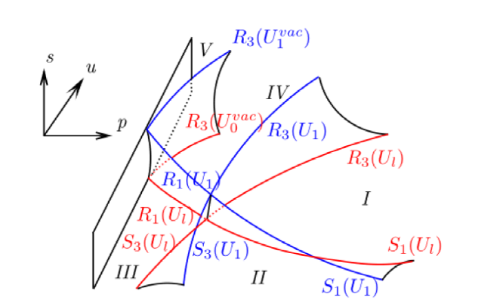
因此基本波将空间 $\{{\Omega}:(p, u, s)\in{\Omega}, p\geq0\}$ 划分为五个部分 (见图 2). 根据右状态 $(p_r, u_r, s_r)$ 所在的区域, 我们构造 (1.1)-(1.3) 式的黎曼解.

(1) 当 $(p_r, u_r, c_r){\in}Ⅰ$ 时, 黎曼解为

$(p_l, u_l, s_l)\xrightarrow{S_1}(p_1, u_1, s_l)\xrightarrow{J_2}(p_1, u_1, s_r)\xrightarrow{R_3}(p_r, u_r, s_r),$

(3.21)

其中 $p_1, u_1$ 满足

$\begin{cases}u_1-u_l=-\varepsilon^\tau{{\rm e}}^{\tau{s_l}/c_v}\sqrt{(p_l^{-2\tau}-p_1^{-2\tau})(p_1-p_l)}, \\ u_r-u_1=\frac{\sqrt{\gamma}\varepsilon^\tau}{\alpha}{\rm e}^{\tau{s_r}/c_v}(p_r^{2\tau\alpha}-p_1^{2\tau\alpha}). \end{cases}$

(3.22)

(2) 当 $(p_r, u_r, c_r){\in}Ⅱ$ 时, 黎曼解为

$(p_l, u_l, s_l)\xrightarrow{S_1}(p_1, u_1, s_l)\xrightarrow{J_2}(p_1, u_1, s_r)\xrightarrow{S_3}(p_r, u_r, s_r),$

(3.23)

其中 $p_1, u_1$ 满足

$\begin{cases}u_1-u_l=-\varepsilon^\tau{{\rm e}}^{\tau{s_l}/c_v}\sqrt{(p_l^{-2\tau}-p_1^{-2\tau})(p_1-p_l)}, \\ u_r-u_1=-\varepsilon^\tau{{\rm e}}^{\tau{s_r}/c_v}\sqrt{(p_1^{-2\tau}-p_r^{-2\tau})(p_r-p_1)}. \end{cases}$

(3.24)

(3) 当 $(p_r, u_r, c_r){\in}Ⅲ$ 时, 黎曼解为

$(p_l, u_l, s_l)\xrightarrow{R_1}(p_1, u_1, s_l)\xrightarrow{J_2}(p_1, u_1, s_r)\xrightarrow{S_3}(p_r, u_r, s_r),$

(3.25)

其中 $p_1, u_1$ 满足

$\begin{cases}u_1-u_l=-\frac{\sqrt{\gamma}\varepsilon^\tau}{\alpha}{\rm e}^{\tau{s_l}/c_v}(p_1^{2\tau\alpha}-p_l^{2\tau\alpha}), \\ u_r-u_1=-\varepsilon^\tau{{\rm e}}^{\tau{s_r}/c_v}\sqrt{(p_1^{-2\tau}-p_r^{-2\tau})(p_r-p_1)}. \end{cases}$

(3.26)

(4) 当 $(p_r, u_r, c_r){\in}Ⅳ$ 时, 黎曼解为

$(p_l, u_l, s_l)\xrightarrow{R_1}(p_1, u_1, s_l)\xrightarrow{J_2}(p_1, u_1, s_r)\xrightarrow{R_3}(p_r, u_r, s_r),$

(3.27)

其中 $p_1, u_1$ 满足

$\begin{cases}u_1-u_l=-\frac{\sqrt{\gamma}\varepsilon^\tau}{\alpha}{\rm e}^{\tau{s_l}/c_v}(p_1^{2\tau\alpha}-p_l^{2\tau\alpha}), \\ u_r-u_1=\frac{\sqrt{\gamma}\varepsilon^\tau}{\alpha}{\rm e}^{\tau{s_r}/c_v}(p_r^{2\tau\alpha}-p_1^{2\tau\alpha}). \end{cases}$

(3.28)

(5) 当 $(p_r, u_r, c_r){\in}Ⅴ$ 时, 黎曼解包含真空状态

$(p_l, u_l, s_l)\xrightarrow{R_1}(0, u_1^{vac}, s_l)\xrightarrow{Vac}(0, u_2^{vac}, s_l)\xrightarrow{J_2}(0, u_2^{vac}, s_r)\xrightarrow{R_3}(p_r, u_r, s_r),$

(3.29)

其中 $u_1^{vac}, u_2^{vac}$ 满足

$\begin{cases}u_1^{vac}=u_l+\frac{\sqrt{\gamma}\varepsilon^\tau}{\alpha}{\rm e}^{\tau{s_l}/c_v}p_l^{2\tau\alpha}, \\ u_2^{vac}=u_r-\frac{\sqrt{\gamma}\varepsilon^\tau}{\alpha}{\rm e}^{\tau{s_r}/c_v}p_r^{2\tau\alpha}. \end{cases}$

(3.30)

4 压力消失时非等熵两相流系统 (1.1)-(1.3) 黎曼解的极限行为

在本节, 我们讨论在压力消失时方程 (1.1)-(1.3) 黎曼解的集中和气穴现象. 当压力消失, 即 $(\varepsilon, \theta)\rightarrow(0, 0)$ 时, 方程 $(3.14)$ 和 $(3.15)$ 都变为

$u=u_l, p>p_l, s=s_l.$

(4.1)

方程 $(3.13)$ 和 $(3.16)$ 都变为

$u=u_l, p<p_l, s=s_l.$

(4.2)

我们可以看出在压力消失过程中区域 $Ⅰ$ 和区域 $Ⅲ$ 逐渐消失. 因此, 我们只需研究 $(p_r, u_r, s_r)\inⅡ, Ⅳ, Ⅴ$ 时方程 (1.1)-(1.3) 黎曼解的极限行为.

4.1 $u_l>u_r$ 时 $\delta$ -激波的形成

接下来, 我们将研究 $(\varepsilon, \theta)\rightarrow(0, 0)$ 且 $(p_r, u_r, s_r)\inⅡ$ 时方程 (1.1)-(1.3) 黎曼解中质量集中现象形成的过程. 对于固定的 $\varepsilon$ 和 $\theta$ , 令 $(p_1^*, u_1^*, s_1^*)$ 和 $(p_2^*, u_2^*, s_2^*)$ 为黎曼解的中间态, 故黎曼解可表示为

$(p_l, u_l, s_l)\xrightarrow{S_1}(p_1^*, u_1^*, s_1^*)\xrightarrow{J_2}(p_2^*, u_2^*, s_2^*)\xrightarrow{S_3}(p_r, u_r, s_r).$

由此可以得到

$\begin{cases}p_1^*=p_2^*, u_1^*=u_2^*, s_1^*=s_l, s_2^*=s_r, \\u_1^*-u_l=-\varepsilon^{\tau}{\rm e}^{{\tau}s_l/c_v}\sqrt{(p_l^{-2\tau}-p_1^{*-2\tau})(p_1^*-p_l)}, \\u_r-u_2^*=-\varepsilon^{\tau}{\rm e}^{{\tau}s_r/c_v}\sqrt{(p_r^{-2\tau}-p_2^{*-2\tau})(p_2^*-p_r)},\end{cases}$

(4.4)

其中, ${\sigma}_1^*, {\sigma}_2^*$ 和 ${\sigma}_3^*$ 分别表示 $S_1, J_2$ 和 $S_3$ 的波速.

接下来, 我们将通过一些引理来说明 $(\varepsilon, \theta)\rightarrow(0, 0)$ 的过程中 $\delta$ -激波的形成.

引理4.1 $\mathop{\lim}\limits_{(\varepsilon, \theta){\rightarrow}(0, 0)}{\rho_1^*}=+\infty, \mathop{\lim}\limits_{(\varepsilon, \theta){\rightarrow}(0, 0)}{\rho_2^*}=+\infty$ .

证将 $(4.4)$ 式的第二个方程和第三个方程相加, 并代入 $p_1^*=p_2^*={\varepsilon}{\rm e}^{s_l/c_v}(\frac{\rho_1^*}{1-\theta{\rho_1^*}})^\gamma$ .

$\begin{matrix} \frac{u_l-u_r}{\sqrt{\varepsilon}{\rm e}^{s_l/(2c_v)}} = &\sqrt{\left(\frac{1}{\rho_l}-\frac{1}{\rho_1^*}\right)\left(\left(\frac{\rho_1^*}{1-\theta\rho_1^*}\right)^\gamma - \left(\frac{\rho_l}{1-\theta\rho_l}\right)^\gamma\right)} \\ + &\sqrt{\left(\frac{1}{\rho_r}-\theta\right) - {\rm e}^{2\tau(s_r-s_l)/c_v}\left(\frac{1}{\rho_1^*}-\theta\right)} \\ &\cdot \sqrt{\left(\left(\frac{\rho_1^*}{1-\theta\rho_1^*}\right)^\gamma - {\rm e}^{(s_r-s_l)/c_v}\left(\frac{\rho_r}{1-\theta\rho_r}\right)^\gamma\right)} \\ = &\left({\frac{\rho_1^*}{1-\theta\rho_1^*}}\right)^{\gamma/2}\left\{\sqrt{\left(\frac{1}{\rho_l}-\frac{1}{\rho_1^*}\right)\left(1-\left(\frac{\rho_l{(1-\theta{\rho_1^*})}}{\rho_1^*{(1-\theta\rho_l)}}\right)^\gamma\right)}\right. \\ &+\sqrt{\left(\frac{1}{\rho_r}-{\rm e}^{2\tau(s_r-s_l)/c_v}\frac{1}{\rho_1^*}\right)-\theta(1-{\rm e}^{2\tau(s_r-s_l)/c_v})} \\ &\left. \cdot\sqrt{\left(1-{\rm e}^{(s_r-s_l)/c_v}\left(\frac{\rho_r(1-\theta\rho_1^*)}{\rho_1^*(1-\theta\rho_r)}\right)^\gamma\right)}\right\}. \end{matrix}$

(4.5)

由 $\rho_1^*>\rho_l$ 可知

$\begin{split}\frac{1}{\rho_l}-\frac{1}{\rho_1^*}, 1-\left(\frac{\rho_l{(1-\theta{\rho_1^*})}}{\rho_1^*{(1-\theta\rho_l)}}\right)^\gamma, \frac{1}{\rho_r}-{\rm e}^{2\tau(s_r-s_l)/c_v}\frac{1}{\rho_1^*}, \\\theta(1-{\rm e}^{2\tau(s_r-s_l)/c_v}), 1-{\rm e}^{(s_r-s_l)/c_v}\left(\frac{\rho_l{(1-\theta{\rho_1^*})}}{\rho_1^*{(1-\theta\rho_l)}}\right)^\gamma,\end{split}$

(4.6)

都是有界值. 即得

$\mathop{\lim}\limits_{(\varepsilon, \theta){\rightarrow}(0, 0)}{\frac{\rho_1^*}{1-\theta\rho_1^*}}=\mathop{\lim}\limits_{(\varepsilon, \theta){\rightarrow}(0, 0)}{\frac{1}{\frac{1}{\rho_1^*}-\theta}}=\mathop{\lim}\limits_{(\varepsilon, \theta){\rightarrow}(0, 0)}{{\rho_1}*}=+\infty.$

(4.7)

再由 ${p_1^*}={p_2^*}$ , 可得

$\mathop{\lim}\limits_{(\varepsilon, \theta){\rightarrow}(0, 0)}{\rho_2^*}=+\infty.$

(4.8)

接下来, 我们计算 $(\varepsilon, \theta)\rightarrow(0, 0)$ 的过程中 $p_1^*$ 的极限.

引理4.2 $\mathop{\lim}\limits_{(\varepsilon, \theta){\rightarrow}(0, 0)}{p_1^*}=\mathop{\lim}\limits_{(\varepsilon, \theta){\rightarrow}(0, 0)}{p_2^*}=\dfrac{\rho_l\rho_r(u_l-u_r)^2}{(\sqrt{\rho_l}+\sqrt{\rho_r})^2}.$

证由方程 $(3.9)$ 可知

$\begin{cases}u_1^*-u_l=-\sqrt{\left(\frac{1}{\rho_1^*}-\frac{1}{\rho_l}\right)(p_l-p_1^*)}, \\u_r-u_2^*=-\sqrt{\left(\frac{1}{\rho_r}-\frac{1}{\rho_2^*}\right)(p_2^*-p_r)}. \end{cases}$

(4.9)

将方程 $(3.9)$ 的第一式与第二式相加可得

$u_r-u_l=-\sqrt{\left(\frac{1}{\rho_1^*}-\frac{1}{\rho_l}\right)(p_l-p_1^*)}-\sqrt{\left(\frac{1}{\rho_r}-\frac{1}{\rho_2^*}\right)(p_2^*-p_r)}.$

(4.9)

取 $(\varepsilon, \theta)\rightarrow(0, 0)$ 时, $(4.10)$ 式两侧的极限, 并代入引理 4.1 的结论, 可得

$u_l-u_r=\left(\frac{1}{\sqrt{\rho_l}}+\frac{1}{\sqrt{\rho_r}}\right)\mathop{\lim}\limits_{(\varepsilon, \theta){\rightarrow}(0, 0)}{\sqrt{p_1^*}}.$

(4.11)

即 $\mathop{\lim}\limits_{(\varepsilon, \theta){\rightarrow}(0, 0)}{p_1^*}=\mathop{\lim}\limits_{(\varepsilon, \theta){\rightarrow}(0, 0)}{p_2^*}=\dfrac{\rho_l\rho_r(u_l-u_r)^2}{(\sqrt{\rho_l}+\sqrt{\rho_r})^2}$ .

引理4.3 令 $\sigma=\dfrac{\sqrt{\rho_l}u_l+\sqrt{\rho_r}u_r}{\sqrt{\rho_l}+\sqrt{\rho_r}}$ , 则有

$\mathop{\lim}\limits_{(\varepsilon, \theta){\rightarrow}(0, 0)}{u_1^*}=\mathop{\lim}\limits_{(\varepsilon, \theta){\rightarrow}(0, 0)}{\sigma_1^*}=\mathop{\lim}\limits_{(\varepsilon, \theta){\rightarrow}(0, 0)}{\sigma_2^*}=\mathop{\lim}\limits_{(\varepsilon, \theta){\rightarrow}(0, 0)}{\sigma_3^*}=\sigma.$

(4.12)

证根据 $(4.10)$ 式和 $(4.11)$ 式可得

$\mathop{\lim}\limits_{(\varepsilon, \theta){\rightarrow}(0, 0)}{u_1^*}=u_l-\mathop{\lim}\limits_{(\varepsilon, \theta){\rightarrow}(0, 0)}{\sqrt{\frac{p_1^*}{\rho_l}}}=\frac{\sqrt{\rho_l}u_l+\sqrt{\rho_r}u_r}{\sqrt{\rho_l}+\sqrt{\rho_r}},$

(4.13)

$\mathop{\lim}\limits_{(\varepsilon, \theta){\rightarrow}(0, 0)}{\sigma_1^*}=\mathop{\lim}\limits_{(\varepsilon, \theta){\rightarrow}(0, 0)}{\frac{\rho_1^*{u_1^*}-{\rho_l}u_l}{\rho_1^*-\rho_l}}=\mathop{\lim}\limits_{(\varepsilon, \theta){\rightarrow}(0, 0)}{\frac{u_1^*-{\rho_l}u_l(\rho_1^*)^{-1}}{1-\rho_l(\rho_1^*)^{-1}}}=\mathop{\lim}\limits_{(\varepsilon, \theta){\rightarrow}(0, 0)}{u_1^*}.$

(4.14)

类似地, 可以得到 $\mathop{\lim}\limits_{(\varepsilon, \theta){\rightarrow}(0, 0)}{\sigma_2^*}=\mathop{\lim}\limits_{(\varepsilon, \theta){\rightarrow}(0, 0)}{\sigma_3^*}=\mathop{\lim}\limits_{(\varepsilon, \theta){\rightarrow}(0, 0)}{u_1^*}=\dfrac{\sqrt{\rho_l}u_l+\sqrt{\rho_r}u_r}{\sqrt{\rho_l}+\rho_r}$ .

引理4.4 质量、动量和焓都是有界的, 即

$\begin{split}&\mathop{\lim}\limits_{(\varepsilon, \theta){\rightarrow}(0, 0)}{\int_{\sigma_1^*}^{\sigma_3^*}{\rho}{\rm d}{\xi}}=\sigma[\rho]-[{\rho}u], \\&\mathop{\lim}\limits_{(\varepsilon, \theta){\rightarrow}(0, 0)}{\int_{\sigma_1^*}^{\sigma_3^*}{({\rho}u)}{\rm d}{\xi}}=\sigma[{\rho}u]-[{\rho}u^2], \\&\mathop{\lim}\limits_{(\varepsilon, \theta){\rightarrow}(0, 0)}{\int_{\sigma_1^*}^{\sigma_3^*}{({\rho}s)}{\rm d}{\xi}}=\sigma[{\rho}s]-[{\rho}us]. \end{split}$

(4.15)

证根据引理 4.1 和引理 4.3, 可以得到

$\begin{split}&\mathop{\lim}\limits_{(\varepsilon, \theta){\rightarrow}(0, 0)}{\int_{\sigma_1^*}^{\sigma_3^*}}{\rho}{\rm d}{\xi}\\=&\mathop{\lim}\limits_{(\varepsilon, \theta){\rightarrow}(0, 0)}{(\rho_2^*(\sigma_3^*-\sigma_2^*)+\rho_1^*(\sigma_2^*-\sigma_1^*))}\\=&\mathop{\lim}\limits_{(\varepsilon, \theta){\rightarrow}(0, 0)}{\left(\rho_2^*{\left(\frac{\rho_r{u_r}-\rho_2^*{u_2^*}}{\rho_r-\rho_2^*}-u_2^*\right)}+\rho_1^*{\left(u_1^*-\frac{\rho_1^*{u_1^*}-{\rho_l}u_l}{\rho_1^*-\rho_l}\right)}\right)}\\=&\mathop{\lim}\limits_{(\varepsilon, \theta){\rightarrow}(0, 0)}{\left(\frac{\rho_2^*\rho_r(u_r-u_2^*)}{\rho_r-\rho_2^*}+\frac{\rho_1^*\rho_l(u_l-u_1^*)}{\rho_1^*-\rho_l}\right)}\\=&\mathop{\lim}\limits_{(\varepsilon, \theta){\rightarrow}(0, 0)}{(\rho_r{s_r}(u_r-u_2^*)+{\rho_l}s_l(u_l-u_1^*))}\\=&\sigma[{\rho}s]-[{\rho}us]. \end{split}$

(4.16)

类似地, 可得

$\begin{split}\mathop{\lim}\limits_{(\varepsilon, \theta){\rightarrow}(0, 0)}{\int_{\sigma_1^*}^{\sigma_3^*}{({\rho}u)}{\rm d}{\xi}}&=\mathop{\lim}\limits_{(\varepsilon, \theta){\rightarrow}(0, 0)}{(\rho_2^*{u_2^*}(\sigma_3^*-\sigma_2^*)+\rho_1^*{u_1^*}(\sigma_2^*-\sigma_1^*))}\\&=\sigma[{\rho}u]-[{\rho}u^2]\end{split}$

(4.17)

和

$\begin{split}\mathop{\lim}\limits_{(\varepsilon, \theta){\rightarrow}(0, 0)}{\int_{\sigma_1^*}^{\sigma_3^*}{({\rho}s)}{\rm d}{\xi}}&=\mathop{\lim}\limits_{(\varepsilon, \theta){\rightarrow}(0, 0)}{(\rho_2^*{s_2^*}(\sigma_3^*-\sigma_2^*)+\rho_1^*{s_1^*}(\sigma_2^*-\sigma_1^*))}\\&=\sigma[{\rho}s]-[{\rho}us]. \end{split}$

(4.18)

引理 4.1-4.4 表明, 当 $(\varepsilon, \theta)\rightarrow(0, 0)$ 时, $S_1, J_2$ 和 $S_3$ 重合到一起, 中间态的密度趋近于无穷大.下面给出以下定理来定量描述 $(\varepsilon, \theta)\rightarrow(0, 0)$ 时质量、动量和焓的集中.

定理4.1 设 $(\rho^{\varepsilon}, u^{\varepsilon}, s^{\varepsilon})$ 为方程 $(1.1)$ - $(1.3)$ 的解, 则当 $u_l>u_r$ 和 $(\varepsilon, \theta)\rightarrow(0, 0)$ 时, 守恒量 $\rho^{\varepsilon}, \rho^{\varepsilon}u^{\varepsilon}$ 和 $\rho^{\varepsilon}s^{\varepsilon}$ 在分布意义下收敛, 且守恒量的极限函数 $\rho, {\rho}u, {\rho}s$ 为阶跃函数和狄拉克函数的和, 它们的权重分别为

$t(\sigma[\rho]-[{\rho}u]), t(\sigma[{\rho}u]-[{\rho}u^2]), t(\sigma[{\rho}s]-[{\rho}us]),$

(4.19)

这与一维常压力流体模型 $(1.4)$ 的黎曼问题中的 $\delta$ -激波解完全相同.

证 $\textbf{(1)}$ 对于 $u_l>u_r$ 和任意的 $\varepsilon>0$ , 方程 (1.1)-(1.3) 的黎曼解为

$(\rho^{\varepsilon}, u^{\varepsilon}, s^{\varepsilon})=\begin{cases}(\rho_l, u_l, s_l), \quad &\xi<\sigma_1^*, \\(\rho_1^*, u_1^*, s_1^*), \quad &\sigma_1^*<\xi<\sigma_2^*, \\(\rho_2^*, u_2^*, s_2^*), \quad &\sigma_2^*<\xi<\sigma_3^*, \\(\rho_r, u_r, s_r), \quad &\xi>\sigma_3^*. \end{cases}$

(4.20)

其中 $(\rho_1^*, u_1^*, s_1^*)$ 和 $(\rho_2^*, u_2^*, s_2^*)$ 为中间状态. 对于任意测试函数 $\varphi(\xi)\in{C_0^{\infty}}$ , (4.20) 式满足

$\int_{-\infty}^{+\infty}{\rho^{\varepsilon}{\varphi}{\rm d}\xi}-\int_{-\infty}^{+\infty}{\rho^{\varepsilon}(u^{\varepsilon}-\xi)\varphi^{'}{\rm d}\xi}=0,$

(4.21a)

$\int_{-\infty}^{+\infty}{\rho^{\varepsilon}u^{\varepsilon}{\varphi}{\rm d}\xi}-\int_{-\infty}^{+\infty}{(\rho^{\varepsilon}u^{\varepsilon}(u^{\varepsilon}-\xi))+p^{\varepsilon}\varphi^{'}{\rm d}\xi}=0,$

(4.21b)

$\int_{-\infty}^{+\infty}{\rho^{\varepsilon}s^{\varepsilon}{\varphi}{\rm d}\xi}-\int_{-\infty}^{+\infty}{(\rho^{\varepsilon}s^{\varepsilon}(u^{\varepsilon}-\xi))\varphi^{'}{\rm d}\xi}=0.$

(4.21c)

$\textbf{(2)}$ 接下来, 根据 $(4.21a)-(4.21c)$ 式求出 $\rho^{\varepsilon}, \rho^{\varepsilon}u^{\varepsilon}, \rho^{\varepsilon}s^{\varepsilon}$ 的极限.

$\textbf{(2a)}$ 对于 (4.21a), 我们将积分项 $\int_{-\infty}^{+\infty}{\rho^{\varepsilon}(u^{\varepsilon}-\xi)\varphi^{'}{\rm d}\xi}$ 分解为四部分

$\left(\int_{-\infty}^{\sigma_1^*}+\int_{\sigma_1^*}^{\sigma_2^*}+\int_{\sigma_2^*}^{\sigma_3^*}+\int_{\sigma_3^*}^{+\infty}\right)(\rho^{\varepsilon}(u^{\varepsilon}-\xi)\varphi^{'}){\rm d}\xi.$

(4.22)

对于 $(4.22)$ 式的第一项和第四项, 可以得到

$\begin{split}&\mathop{\lim}\limits_{(\varepsilon, \theta){\rightarrow}(0, 0)}{\left(\int_{-\infty}^{\sigma_1^*}+\int_{\sigma_3^*}^{+\infty}\right)\rho^{\varepsilon}(u^{\varepsilon}-\xi)\varphi^{'}{\rm d}\xi}\\=&(\sigma[\rho]-[\rho{u}])\varphi(\sigma)+\int_{-\infty}^{+\infty}{H(\xi-u_{\delta})\varphi{{\rm d}\xi}},\end{split}$

(4.23)

其中

$H(\xi-u_{\delta})=\begin{cases}\rho_l, \quad &\xi<u_{\delta}, \\\rho_r, \quad &\xi>u_{\delta}. \end{cases}$

对于 $(4.22)$ 式的第二部分, 可以得到

$\begin{split}&\mathop{\lim}\limits_{(\varepsilon, \theta){\rightarrow}(0, 0)}{\int_{\sigma_1^*}^{\sigma_2^*}\rho^{\varepsilon}(u^{\varepsilon}-\xi)\varphi^{'}{\rm d}\xi}=\mathop{\lim}\limits_{(\varepsilon, \theta){\rightarrow}(0, 0)}{\int_{\sigma_1^*}^{\sigma_2^*}\rho_1^*(u_1^*-\xi)\varphi^{'}{\rm d}\xi}\\=&\mathop{\lim}\limits_{(\varepsilon, \theta){\rightarrow}(0, 0)}{\left\{{\rho_1^*}u_1^*(\varphi(\sigma_2^*)-\varphi(\sigma_1^*))-\rho_1^*(\sigma_2^*\varphi(\sigma_2^*)-\sigma_1^*\varphi(\sigma_1^*))+\rho_1^*\int_{\sigma_1^*}^{\sigma_2^*}\varphi(\xi){\rm d}{\xi}\right\}}\\=&\mathop{\lim}\limits_{(\varepsilon, \theta){\rightarrow}(0, 0)}\left\{\rho_1^*({\sigma_2^*}-{\sigma_1^*})\left({u_1^*}\frac{\varphi(\sigma_2^*)-\varphi(\sigma_1^*)}{\sigma_2^*-\sigma_1^*}-\frac{{\sigma_2^*}\varphi(\sigma_2^*)-\sigma_1^*\varphi(\sigma_1^*)}{{\sigma_2^*}-{\sigma_1^*}}+\frac{\int_{\sigma_1^*}^{\sigma_2^*}\varphi(\xi){\rm d}\xi}{{\sigma_2^*}-{\sigma_1^*}}\right)\right\}\\=&-{\rho_l}(\sigma-u_l)(\sigma\varphi^{'}(\sigma)-\sigma\varphi^{'}(\sigma)-\varphi(\sigma)+\varphi(\sigma))\\=&0. \end{split}$

(4.25)

同样地, 对于 $(4.22)$ 式的第三部分, 计算可得

$\mathop{\lim}\limits_{(\varepsilon, \theta){\rightarrow}(0, 0)}{\int_{\sigma_2^*}^{\sigma_3^*}}{\rho^{\varepsilon}(u^{\varepsilon}-\xi)\varphi^{'}{\rm d}\xi}=0.$

(4.26)

然后, 通过将 $(4.23), (4.25)$ 和 $(4.26)$ 式代入 $(4.21a)$ 式得到

$\mathop{\lim}\limits_{(\varepsilon, \theta){\rightarrow}(0, 0)}{\rho^{\varepsilon}{\varphi}{\rm d}\xi}=(\sigma[\rho]-[\rho{u}])\varphi(\sigma)+\int_{-\infty}^{+\infty}{H(\xi-u_{\delta})\varphi{{\rm d}\xi}},$

(4.27)

其中, $\varphi\in{C_0^{\infty}}$ 是任意的测试函数.

$\textbf{(2b) }$ 对于 $(4.21b)$ , 如上可证

$\begin{split}&\mathop{\lim}\limits_{(\varepsilon, \theta){\rightarrow}(0, 0)}{\rho^{\varepsilon}u^{\varepsilon}(u^{\varepsilon}-\xi)\varphi^{'}{\rm d}\xi}\\=&(\sigma[\rho{u}]-[\rho{u^2}])\varphi(\sigma)+\int_{-\infty}^{+\infty}{H_1(\xi-u_{\delta})\varphi{{\rm d}\xi}}. \end{split}$

(4.28)

其中

$H_1(\xi-u_{\delta})=\begin{cases}\rho_l{u_l}, \quad &\xi<u_{\delta}, \\\rho_r{u_r}, \quad &\xi>u_{\delta}. \end{cases}$

(4.29)

此外, 根据引理 4.2 和 4.3, 可得

$\begin{split}&\mathop{\lim}\limits_{(\varepsilon, \theta){\rightarrow}(0, 0)}{\int_{-\infty}^{+\infty}}{p^{\varepsilon}\varphi^{'}{\rm d}\xi}\\=&\mathop{\lim}\limits_{(\varepsilon, \theta){\rightarrow}(0, 0)}\left\{{\int_{-\infty}^{\sigma_1^*}+\int_{\sigma_1^*}^{\sigma_2^*}+\int_{\sigma_2^*}^{\sigma_3^*}+\int_{\sigma_3^*}^{+\infty}}\right\}p^{\varepsilon}\varphi^{'}{\rm d}\xi\\=&\mathop{\lim}\limits_{(\varepsilon, \theta){\rightarrow}(0, 0)}\{p_l\varphi(\sigma_1^*)+p_1^*(\sigma_2^*-\sigma_1^*)+p_2^*(\sigma_3^*-\sigma_2^*)+p_r\varphi(\sigma_3^*)\}\\=&0. \end{split}$

(4.30)

综上所述, 可得

$\mathop{\lim}\limits_{(\varepsilon, \theta){\rightarrow}(0, 0)}{\rho^{\varepsilon}u^{\varepsilon}\varphi{{\rm d}\xi}}=(\sigma[\rho{u}]-[\rho{u^2}])\varphi(\sigma)+\int_{-\infty}^{+\infty}{H_1(\xi-u_{\delta})\varphi{{\rm d}\xi}}.$

(4.31)

$\textbf{(2c) }$ 对于 (4.21c), 用同样的分解方法可以得到

$\begin{split}&\int_{-\infty}^{+\infty}{\rho^{\varepsilon}s^{\varepsilon}(u^{\varepsilon}-\xi)\varphi^{'}{\rm d}\xi}\\=&\left(\int_{-\infty}^{\sigma_1^*}+\int_{\sigma_1^*}^{\sigma_2^*}+\int_{\sigma_2^*}^{\sigma_3^*}+\int_{\sigma_3^*}^{+\infty}\right)(\rho^{\varepsilon}s^{\varepsilon}(u^{\varepsilon}-\xi)\varphi^{'}){\rm d}\xi. \end{split}$

(4.32)

并且 $(4.32)$ 式等号右边的第一项和第四项之和的极限是

$\begin{split}&\mathop{\lim}\limits_{(\varepsilon, \theta){\rightarrow}(0, 0)}{\left(\int_{-\infty}^{\sigma_1^*}+\int_{\sigma_3^*}^{+\infty}\right)}\rho^{\varepsilon}s^{\varepsilon}(u^{\varepsilon}-\xi)\varphi^{'}{\rm d}\xi\\=&(\sigma[\rho{s}]-[\rho{us}])\varphi(\sigma)+\int_{-\infty}^{+\infty}H_2(\xi-u_{\delta})\varphi{{\rm d}\xi}. \end{split}$

(4.33)

其中

$H_2(\xi-u_{\delta})\begin{cases}\rho_l{s_l}, \quad &\xi<u_{\delta}, \\\rho_r{s_r}, \quad &\xi>u_{\delta}. \end{cases}$

(4.34)

此外, $(4.32)$ 式等号右边的第二项和第三项之和的极限是

$\begin{split}&\mathop{\lim}\limits_{(\varepsilon, \theta){\rightarrow}(0, 0)}{\left(\int_{\sigma_1^*}^{\sigma_2^*}+\int_{\sigma_2^*}^{\sigma_3^*}\right)}{\rho^{\varepsilon}s^{\varepsilon}(u^{\varepsilon}-\xi)\varphi^{'}{\rm d}\xi}\\=&\mathop{\lim}\limits_{(\varepsilon, \theta){\rightarrow}(0, 0)}{\int_{\sigma_1^*}^{\sigma_2^*}}{\rho_1^*{s_l}(u_1^*-\xi)\varphi^{'}{\rm d}\xi}+\mathop{\lim}\limits_{(\varepsilon, \theta){\rightarrow}(0, 0)}{\int_{\sigma_2^*}^{\sigma_3^*}}{\rho_2^*{s_r}(u_2^*-\xi)\varphi^{'}{\rm d}\xi}\\=&0. \end{split}$

(4.35)

因此, 可以得到

$\mathop{\lim}\limits_{(\varepsilon, \theta){\rightarrow}(0, 0)}{\int_{-\infty}^{+\infty}}{\rho^{\varepsilon}s^{\varepsilon}\varphi{{\rm d}\xi}}=(\sigma[\rho{s}]-[\rho{us}])\varphi(\sigma)+\int_{-\infty}^{+\infty}{H_2(\xi-u_{\delta})\varphi{{\rm d}\xi}}.$

(4.36)

$\textbf{(3) }$ 接下来, 我们讨论当 $(\varepsilon, \theta)\rightarrow(0, 0)$ 时 $\rho^{\varepsilon}, \rho^{\varepsilon}u^{\varepsilon}, \rho^{\varepsilon}s^{\varepsilon}$ 在分布意义下的极限. 对于任意的 $\psi(t, x)\in{C_0^{\infty}}(\mathbb{R}^{+}\times\mathbb{R})$ , 有

$\begin{split}&\mathop{\lim}\limits_{(\varepsilon, \theta){\rightarrow}(0, 0)}{\int_{0}^{+\infty}}\int_{-\infty}^{+\infty}{\rho^{\varepsilon}(t, x)\psi(t, x){\rm d}x{\rm d}t}\\=&\mathop{\lim}\limits_{(\varepsilon, \theta){\rightarrow}(0, 0)}{\int_{0}^{+\infty}}\int_{-\infty}^{+\infty}{\rho^{\varepsilon}(\xi)\psi(t, \xi{t})t{\rm d}{\xi}{\rm d}t}\\=&\int_{0}^{+\infty}t\left((\sigma[\rho]-[\rho{u}])\psi(t, \sigma{t})+\int_{-\infty}^{+\infty}\rho_0\psi(t, \xi{t}){\rm d}\xi\right){\rm d}t\\=&\int_{0}^{+\infty}\int_{-\infty}^{+\infty}\rho_0{\psi(t, x){\rm d}x{\rm d}t}+\langle\omega_1(t)\delta_{S}, \psi(t, \sigma{t})\rangle,\end{split}$

(4.37)

其中

$\omega_1(t)=t(\sigma[\rho]-[\rho{u}]),$

这和 $(2.10)$ 式相同. 类似地, 可以求出

$\begin{split}&\mathop{\lim}\limits_{(\varepsilon, \theta){\rightarrow}(0, 0)}{\int_{0}^{+\infty}\int_{-\infty}^{+\infty}}\rho^{\varepsilon}{(t, x)}u^{\varepsilon}(t, x)\psi(t, x){\rm d}x{\rm d}t\\=&\int_{0}^{+\infty}\int_{-\infty}^{+\infty}\rho_0{u_0}\psi(t, x){\rm d}x{\rm d}t+\langle\omega_2(t)\delta_S, \psi(t, \sigma{t})\rangle\end{split}$

(4.39)

和

$\begin{split}&\mathop{\text{lim}}\limits_{(\varepsilon, \theta){\rightarrow}(0, 0)}{\int_{0}^{+\infty}\int_{-\infty}^{+\infty}}\rho^{\varepsilon}{(t, x)}s^{\varepsilon}(t, x)\psi(t, x){\rm d}x{\rm d}t\\=&\int_{0}^{+\infty}\int_{-\infty}^{+\infty}\rho_0{s_0}\psi(t, x){\rm d}x{\rm d}t+\langle\omega_3(t)\delta_S, \psi(t, \sigma{t})\rangle,\end{split}$

(4.40)

其中

$\omega_2(t)=t(\sigma[\rho{u}]-[\rho{u^2}]), \omega_3(t)=t(\sigma[\rho{s}]-[\rho{u}s]).$

(4.41)

4.2 $u_l<u_r$ 时真空的形成

接下来, 我们将研究当 $(\varepsilon, \theta)\rightarrow(0, 0)$ 时, 方程 (1.1)-(1.3) 的黎曼解极限中气穴现象的形成. 此处, 要求 $(p_r, u_r, s_r)\inⅣ, Ⅴ$ 且 $u_l<u_r$ . 当 $(p_r, u_r, s_r)\inⅣ$ 时, 对任意的 $\varepsilon$ , 方程 (1.1)-(1.3) 的黎曼解可表示为

$(p_l, u_l, s_l)\xrightarrow{R_1}(p_1^*, u_1^*, s_1^*)\xrightarrow{J_2}(p_2^*, u_2^*, s_2^*)\xrightarrow{R_3}(p_r, u_r, s_r),$

(4.42)

其中 $(p_1^*, u_1^*, s_1^*)$ 和 $(p_2^*, u_2^*, s_2^*)$ 为中间状态. 根据 $(3.13)$ 式和 $(3.15)$ 式可以得到

$\begin{cases}p_1^*=p_2^*, u_1^*=u_2^*, s_1^*=s_l, s_2^*=s_r, \\u_1^*-u_l=-\frac{\sqrt{\gamma}\varepsilon^{\tau}}{\alpha}{\rm e}^{{\tau}s_l/c_v}(p_1^{*2\tau\alpha}-p_l^{2\tau\alpha}), \\u_r-u_2^*=\frac{\sqrt{\gamma}\varepsilon^{\tau}}{\alpha}{\rm e}^{{\tau}s_r/c_v}(p_r^{2\tau\alpha}-p_2^{*2\tau\alpha}). \end{cases}$

(4.43)

将 $(4.43)$ 式的第二项和第三项相加可以得到

$\begin{split}u_r-u_l&=\frac{\sqrt{\gamma{\varepsilon}^{\tau}}}{\alpha}\left({\rm e}^{\tau{s_l/c_v}}p_l^{2\tau\alpha}+{\rm e}^{\tau{s_r/c_v}}p_r^{2\tau\alpha}-\left({\rm e}^{\tau{s_l/c_v}}+{\rm e}^{\tau{s_r/c_v}}\right)p_1^{*2\tau\theta}\right)\\&<\frac{\sqrt{\gamma}\varepsilon^{\tau}}{\alpha}\left({\rm e}^{\tau{s_l/c_v}}p_l^{2\tau\alpha}+{\rm e}^{\tau{s_r/c_v}}p_r^{s2\tau\alpha}\right)\\&=\frac{\sqrt{\gamma\varepsilon}}{\alpha}\left({\rm e}^{s_l/2c_v}\left(\frac{\rho_l}{1-\theta\rho_l}\right)^{\alpha}+{\rm e}^{s_r/2c_v}\left(\frac{\rho_r}{1-\theta\rho_r}\right)^{\alpha}\right). \end{split}$

(4.44)

由上可得以下引理.

引理4.5 若 $\varepsilon$ 和 $\theta$ 满足

$\frac{\alpha^{2}(u_r-u_l)^2}{\varepsilon\gamma\left({\rm e}^{s_l/2c_v}\left(\frac{\rho_l}{1-\theta\rho_l}\right)^{\alpha}+{\rm e}^{s_r/2c_v}\left(\frac{\rho_r}{1-\theta\rho_r}\right)^{\alpha}\right)^2}<1,$

(4.45)

方程 (1.1)-(1.3) 的黎曼解不会出现真空. 若 (4.45) 式被违反, 方程 (1.1)-(1.3) 的黎曼解必然出现真空.

注4.1 由引理 4.5 可知, 对于任意的 $(\rho_r, u_r, s_r)$ , 如果 $\varepsilon, \theta$ 充分小, 它对应的初值 $(p_r, u_r, s_r)$ 属于区域 $V$ . 当 $\varepsilon<\varepsilon_0$ 时, 方程 (1.1)-(1.3) 的黎曼解包含真空状态可以表示为

$(\rho^{\varepsilon}, u^{\varepsilon}, s^{\varepsilon})=\begin{cases}(\rho_l, u_l, s_l),&\xi<\lambda_1(\rho_l, u_l, s_l), \\(\rho_(\xi), u_(\xi), s_l),&\lambda_1(\rho_l, u_l, s_l)<\xi<u_1^{vac}, \\(0, u(\xi), s(\xi)),&u_1^{vac}<\xi<u_2^{vac}, \\(\rho_(\xi), u_(\xi), s_r),&u_2^{vac}<\xi<\lambda_3(\rho_r, u_r, s_r), \\(\rho_r, u_r, s_r),&\xi>\lambda_3(\rho_r, u_r, s_r),\end{cases}$

其中

$u_1^{vac}=u_l+\frac{\sqrt{\varepsilon\gamma}{{\rm e}^{s_l/2c_v}}}{\alpha}(\frac{\rho_l}{1-\theta\rho_l})^{\alpha},u_2^{vac}=u_r-\frac{\sqrt{\varepsilon\gamma}{{\rm e}^{s_r/2c_v}}}{\alpha}(\frac{\rho_r}{1-\theta\rho_r})^{\alpha}.$

(4.47)

由 (4.47) 式可知

$\begin{split}\mathop{\text{lim}}\limits_{(\varepsilon, \theta){\rightarrow}(0, 0)}&\lambda_1(\rho_l, u_l, s_l)=\mathop{\text{lim}}\limits_{(\varepsilon, \theta){\rightarrow}(0, 0)}u_1^{vac}=u_l, \\\mathop{\text{lim}}\limits_{(\varepsilon, \theta){\rightarrow}(0, 0)}&\lambda_3(\rho_r, u_r, s_r)=\mathop{\text{lim}}\limits_{(\varepsilon, \theta){\rightarrow}(0, 0)}u_2^{vac}=u_r,\end{split}$

(4.48)

从上述分析中, 可以知道当 $(\varepsilon, \theta)\rightarrow(0, 0)$ 时, 第一族稀疏波逐渐收敛成特征速度为 $u_l$ 的接触间断. 类似地, 第三族稀疏波逐渐收敛成特征速度为 $u_r$ 的接触间断. 同时, 真空状态持续膨胀, 直至充满两个接触间断之间的区域. 因此, 可以得出以下结论.

定理4.2 对于 $u_l<u_r$ , 当 $(\varepsilon, \theta)\rightarrow(0, 0)$ 时, 方程 (1.1)-(1.3) 的黎曼解 $(\rho^{\varepsilon}, u^{\varepsilon}, s^{\varepsilon})$ 的极限为

$(\rho, u, s)=\begin{cases}(\rho_l, u_l, s_l), \quad &\xi<u_l, \\(0, u(\xi), s(\xi)), \quad &u_l<\xi<u_r, \\(\rho_r, u_r, s_r), \quad &\xi>u_r,\end{cases}$

(4.49)

这与一维常压力流体模型 $(1.4)$ 的黎曼问题中的真空解完全相同.

5 数值模拟

本节将利用 ENO 格式和三阶 Runge-Kutta 对系统 (1.1)-(1.3) 进行数值模拟, 其中网格单元划分为 $60\times60$ , CFL=0.4.

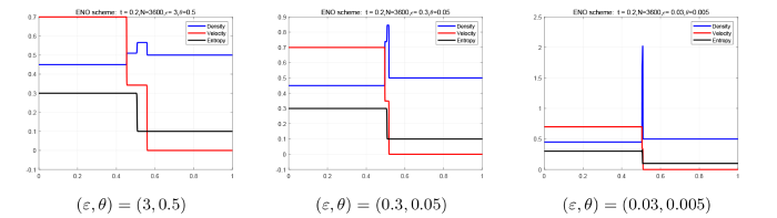
5.1 $\delta$ -激波的数值模拟

在本小节中, 我们取初值为

$(\rho, u, s)|_{t=0}=\begin{cases}(0.5, 0, 0.1)\quad &x<0, \\(0.45, 0.7, 0.3)\quad &x>0. \end{cases}$

(5.1)

图 3 展示了当 $t=0.2$ 时, 参数 $\varepsilon, \theta$ 取不同值时的黎曼解, 其中红线、蓝线和黑线分别表示密度、速度和熵. 该过程显示了 $\delta$ -激波的形成. 从图 3 中可以看出, 当 $(\varepsilon, \theta)\rightarrow(0, 0)$ 时, 速度 $u$ 和熵 $s$ 变成阶跃函数, 中间态密度急剧增加.这一现象完全符合定理 4.1.

图3

新窗口打开| 下载原图ZIP| 生成PPT

图3 $(\varepsilon, \theta)$ 取不同值时方程 (1.1) 和 (5.1) 的黎曼解

5.2 真空状态的数值模拟

在本小节中, 我们取初值为

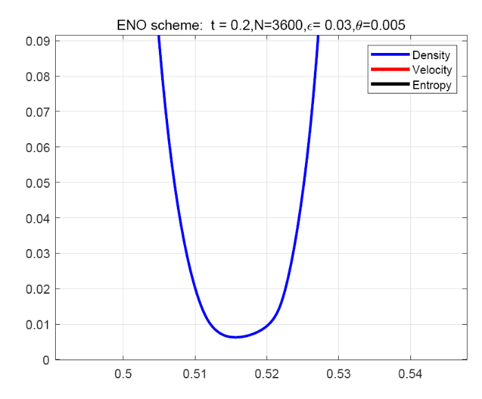
$(\rho, u, s)|_t=\begin{cases}(0.5, 1.5, 0.1)\quad &x<0, \\(0.45, 0.1, 0.3)\quad &x>0. \end{cases}$

(5.2)

图 4 展示了当 $t=0.2$ 时, 参数 $\varepsilon, \theta$ 取不同值时的黎曼解, 其中红线、蓝线和黑线分别表示密度、速度和熵. 该过程显示了真空状态的形成. 此外, 图 5 为 $(\varepsilon, \theta)=(0.03, 0.005)$ 时密度细节的放大图. 从图 4 和图 5 中可以看出, 当 $(\varepsilon, \theta)\rightarrow(0, 0)$ 时, 中间态的密度逐渐减小并无限接近于 $0$ , 但没有出现真空. 同时, 速度 $u$ 和熵 $s$ 从阶跃函数过度到连续函数. 之后, 真空状态的区域持续膨胀, 填满两个接触间断之间的区域. 这一现象完全符合定理 4.1.

图4

新窗口打开| 下载原图ZIP| 生成PPT

图4 $(\varepsilon, \theta)$ 取不同值时方程 (1.1) 和 (5.2) 的黎曼解

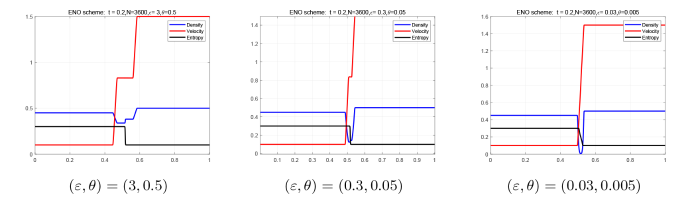
图5

新窗口打开| 下载原图ZIP| 生成PPT

图5 $(\varepsilon, \theta)=(0.03, 0.005)$ 时方程 (1.1) 和 (5.2) 黎曼解中密度的局部细节

参考文献

原文顺序

文献年度倒序

文中引用次数倒序

被引期刊影响因子

[1]

Bereux

, Bonnetier

, LeFloch

P G

Gas dynamics system: two special cases

SIAM Journal on Mathematical Analysis, 1997, 28(3): 499-515

[本文引用: 2]

[2]

Bilicki

, Kestin

Physical aspects of the relaxation model in two-phase flow

Proceedings of the Royal Society of London A Mathematical and Physical Sciences, 1990, 428(1875): 379-397