Processing math: 0%

数学物理学报, 2025, 45(1): 180-188

随机扰动下三阶MQ拟插值在导数逼近中的应用研究

张胜良,1,*, 钱艳艳,2

1南京林业大学经济管理学院 南京 210037

2南京林业大学理学院 南京 210037

Application of Cubic MQ Quasi-Interpolation in Derivative Approximations Under Random Perturbation

Zhang Shengliang,1,*, Qian Yanyan,2

1College of Economics and Management, Nanjing Forestry University, Nanjing 210037

2College of Science, Nanjing Forestry University, Nanjing 210037

通讯作者: * 张胜良,E-mail:10110180035@fudan.edu.cn

收稿日期: 2024-03-22   修回日期: 2024-07-9  

基金资助: 教育部人文社会科学研究 `基于两种市场决策机制的林业碳汇价值评估研究-实物期权模型的改进与应用'项目(21YJC790162)
江苏省社科基金 "双碳" 目标下苏北杨树产业碳汇价值实现机制及支持政策研究(22EYB010)

Received: 2024-03-22   Revised: 2024-07-9  

Fund supported: Improvement and application of real option model'(21YJC790162)
Jiangsu Provincial Social Science Foundation(22EYB010)

作者简介 About authors

钱艳艳,E-mail:qianyanyan@njfu.edu.cn

摘要

该文基于三阶 MQ (multiquadric) 拟插值算子, 提出了在随机扰动背景下有效逼近高阶导数的数值方法, 并给出了相应的数值算例和误差估计. 试验表明, 该方法相比已有方法精度更高、更稳定、更有效.

关键词: 导数逼近; 随机扰动; MQ 拟插值; 误差估计.

Abstract

This paper proposes a numerical method that can effectively approximate high-order derivatives under random perturbation based on the cubic MQ (multiquadric) quasi-interpolation operator. Corresponding numerical examples and error estimates are given. Numerical experimental results show that the proposed method is more accurate, more stable and more effective than the existing methods.

Keywords: derivative approximation; random perturbation; multi-quadric quasi-interpolation; error estimations.

PDF (965KB) 元数据 多维度评价 相关文章 导出 EndNote| Ris| Bibtex  收藏本文

本文引用格式

张胜良, 钱艳艳. 随机扰动下三阶MQ拟插值在导数逼近中的应用研究[J]. 数学物理学报, 2025, 45(1): 180-188

Zhang Shengliang, Qian Yanyan. Application of Cubic MQ Quasi-Interpolation in Derivative Approximations Under Random Perturbation[J]. Acta Mathematica Scientia, 2025, 45(1): 180-188

1 引言

高阶导数逼近在科学、工程和应用数学等领域具有关键作用, 对于理解、模拟和优化复杂系统以及解决许多实际问题至关重要. 但在求解高阶导数问题时, 有限差分法 (Finite Difference Method, FDM)、有限元法和谱方法等数值方法由于它们复杂的数值格式构造和计算网格划分导致在实际应用中受到一定的限制. 与这些方法相比, 无网格方法对边界条件和初始条件有更强的适应性, 在处理高维问题方面也具有特殊优势. 其中一种无网格方法是利用径向基函数 (Radial Basis Function, RBF) 逼近高阶导数.

MQ 函数是 RBF 中的重要一类, 由于它计算简单、各向同性等优点, 被广泛应用于数值计算, 最早是由 Hardy [10] 在解决航天器外形设计的问题时于 1971 年提出. MQ 函数插值采用 ϕ(x)= 作为核函数, \left\{ {{\phi _j}(x - {x_j})} \right\} 作为一组基函数, 使得 s({x_k}) = \sum {{\lambda _j}\phi ({x_k} - {x_j})} = {f_k}. 因此插值方法一般会涉及系数矩阵是否可逆的问题, 为了避免对条件数很大的矩阵求逆, 拟插值方法应运而生. 它在满足理想精度的同时可以直接对函数赋值, 不需要对矩阵求逆. 因此, MQ 拟插值算法受到了大量研究者的关注并得到广泛应用.

理论方面, Franke[7] 通过实验比较得出 MQ 拟插值在精度和稳定性等方面均表现较好; Buhmann[2] 研究了 MQ 拟插值的收敛性问题; Beatson 和 Powell [1]构造了三种有界区间上的 MQ 拟插值算子, 记作 {L_A}{L_B}{L_C}; Wu 和 Schaback [15] 在此基础上构造了一种不需要导数信息且具备保形性的新算子 {L_D}. 应用方面, MQ 拟插值不仅在求解微分方程上[3,5,11,14,16,18] 有突出表现, 而且在计算机辅助设计[8]、经济学 [17] 等领域也发挥着重要作用.

在处理大规模、高维度数据时, 现有的 MQ 方法时常难以提供足够的精确度. 这不仅会导致多步数值计算时的累积误差增大, 还会引发数值不稳定性问题, 造成数值溢出或数值精度丧失的情况. 为应对这一挑战, 本文在随机扰动的背景下, 研究有效逼近高阶导数的高精度方法. 通过加入噪声, 能更准确地模拟实际数据. 相比于传统的 MQ 拟插值方法, 高精度的三阶 MQ 拟插值能够更好地拟合数据的非线性特征, 具有更高的稳定性, 可以处理更广泛的随机数据逼近问题.

具体来说, 给定一个序列

{\rm X} = \cdots < {x_{i - 1}} < {x_i} < {x_{i + 1}} < \cdots, \begin{array}{*{20}{c}} {}&{h \equiv \mathop {\max }\limits_i ({x_i} - {x_{i - 1}}).} \end{array}

i \to \pm \infty 时, {x_{ \pm i}} \to \pm \infty . 函数 f:\mathbb{R} \mapsto \mathbb{R} 在序列 {\rm X} 上的三阶 MQ 拟插值具有形式

\begin{equation} ({\cal L}f) = \sum {f({x_i})} {\Phi _i}(x), \end{equation}
(1.1)

其中

{\Phi _i}(x) = \Phi (x - {x_i}) = \frac{{{\varphi _{i + 1}}(x) - {\varphi _i}(x)}}{{2({x_{i + 2}} - {x_{i - 1}})}} - \frac{{{\varphi _i}(x) - {\varphi _{i - 1}}(x)}}{{2({x_{i + 1}} - {x_{i - 2}})}}.

这里 {\varphi _i}(x) 是三阶 MQ 函数的线性组合, 具体形式如下所示

\varphi_{i}(x)=\varphi\left(x-x_{i}\right)=\frac{\left(\phi_{i+1}-\phi_{i}\right) /\left(x_{i+1}-x_{i}\right)-\left(\phi_{i}-\phi_{i-1}\right) /\left(x_{i}-x_{i-1}\right)}{x_{i+1}-x_{i-1}},

这里 \phi (x) = \sqrt {{{({x^2} + {c^2})}^3}} {\phi _i}(x) = \sqrt {{{((x - {x_i})}^2} + {c^2}{)^3}} , 其中 c 为形状参数. 文献 [1] 给出了上述拟插值保单调性和保凸性的证明. 本文将对随机扰动下三阶 MQ 拟插值算子的逼近阶进行理论和试验证明.

本文主要结构如下. 在第 2 节, 我们给出了三阶 MQ 拟插值性质的一些理论证明, 并在随机扰动背景下分析了它对高阶导数的逼近阶. 在第 3 节, 针对一元、多元和偏微分方程数值解中的具体应用分别给出算例和误差估计. 第 4 节进行简单总结.

2 三阶 MQ 拟插值方法

在测量或者采样中, 样本数据总是不可避免地带有误差. 为了更接近真实情况, 本文对采样点数据值加入一定的噪声来模拟测量采样或计算机精度所造成的误差, 即 { {\hat f({x_i}) = f({x_i}) + {e_i}} }, 其中 {e_i} 是随机误差. 问题形式上就演变成用带有随机误差项的采样值 \hat f({x_i}) 去估计高阶导数 {f^{(n)}}(x). 这里假设 {e_i} 为白噪声, E(e)、Var(e) 分别表示随机变量 {e_i} 的均值和方差. 满足

\begin{equation} \left\{ {\begin{array}{*{20}{l}} {E({e_i}) = 0},\\ {{\rm Var}({e_i}) = {\sigma _i}^2},\\ {{\mathop{\rm cov}} ({e_i},{e_j}) = 0,i \ne j}. \end{array}} \right. \end{equation}
(2.1)

在讨论之前还需要做一些理论准备. 由文献 [12,13]经过推导可分别得出如下引理2.1, 2.2.

引理2.1 如果 f(x) \in {C^{(n + 4)}}(\mathbb{R})\left| {{f^{(i)}}(x)} \right| 小于某 n + 4 - i 次多项式, 那么有

\begin{equation} \left| {({\cal L}{f^{(n)}})(x) - {f^{(n)}}(x)} \right| < {\cal O}({h^{{\textstyle{4 \over {n + 3}}}}}), n \ge 2. \end{equation}
(2.2)

引理2.2 不等式

\begin{equation} \int_{ - \infty }^{ + \infty } {{{[{\phi ^{(n)}}(x)]}^2}{\rm d}x \le } {\cal O}\left( {\frac{1}{{{c^{2n - 7}}}}} \right) \end{equation}
(2.3)

成立.

现在对三阶 MQ 拟插值在随机扰动背景下对高阶导数的逼近能力进行分析. 有如下定理

定理2.1 如果取 c = {\cal O}({h^{{\textstyle{1 \over {n + 3}}}}}), 那么利用三阶 MQ 拟插值估计 n 阶导数算子 {\cal L} 的误差为

\begin{equation}\label{eq:q1} E{[({\cal L}{\hat f^{(n)}})(x) - {f^{(n)}}(x)]^2} \le {\cal O}(\frac{{{{\bar \sigma }^2}}}{{{h^{{\textstyle{{n - 2} \over {n + 3}}}}}}}) + {\cal O}({h^{{\textstyle{8 \over {n + 3}}}}}), \end{equation}
(2.4)

这里 {\bar \sigma ^2}: = \mathop {\max }\limits_i \sigma _i^2, \hat ff 引入随机干扰后的三阶 MQ 拟插值逼近.

计算有

\begin{array}{l} ~~~\,E{[({\cal L}{{\hat f}^{(n)}})(x) - {f^{(n)}}(x)]^2}\\ = E{[({\cal L}{{\hat f}^{(n)}})(x) + {({\cal L}f)^{(n)}}(x) - {({\cal L}f)^{(n)}}(x) - {f^{(n)}}(x)]^2}\\ = E\bigg[\sum\limits_{i = - \infty }^{ + \infty } {\hat f({x_i})\Phi _i^{(n)}(x)} + \sum\limits_{i = - \infty }^{ + \infty } {f({x_i})\Phi _i^{(n)}(x)} - \sum\limits_{i = - \infty }^{ + \infty } {f({x_i})\Phi _i^{(n)}(x)} - {f^{(n)}}\bigg]. \end{array}

注意

E\bigg[\sum\limits_{i = - \infty }^{ + \infty } {\hat f({x_i})\Phi _i^{(n)}(x)} - \sum\limits_{i = - \infty }^{ + \infty } {f({x_i})\Phi _i^{(n)}(x)} \bigg] = 0,

于是

\begin{array}{l} ~~~\,E{[({\cal L}{{\hat f}^{(n)}})(x) - {f^{(n)}}(x)]^2}\\ ={\bigg[\sum\limits_{i = - \infty }^{ + \infty } {f({x_i})\Phi _i^{(n)}(x)} - {f^{(n)}}(x)\bigg]^2} + E{\bigg[\sum\limits_{i = - \infty }^{ + \infty } {\hat f({x_i})\Phi _i^{(n)}(x)} - \sum\limits_{i = - \infty }^{ + \infty } {f({x_i})\Phi _i^{(n)}(x)} \bigg]^2}. \end{array}

由于

{\Phi _i}(x) = {[{x_{i - 2}},{x_{i - 1}},{x_{i,}}{x_{i + 1}},{x_{i + 2}}]_v}\phi (x - v)\frac{{{x_{i + 2}} - {x_{i - 2}}}}{2} = \frac{{{x_{i + 2}} - {x_{i - 2}}}}{4} \cdot \frac{{{\phi ^{(4)}}(x - {u_i})}}{{12}},

这里{u_i} \in [{x_{i - 2}},{x_{i + 2}}], 同时根据引理2.1, 我们有

\begin{align*} E{[({\cal L}{{\hat f}^{(n)}})(x) - {f^{(n)}}(x)]^2} & \le \mathop {\max }\limits_i \sigma _i^2\sum\limits_{i = - \infty }^{ + \infty } {{{[\Phi _i^{(n)}(x)]}^2}} + {\cal O}{({h^{{\textstyle{4 \over {n + 3}}}}})^2}\\ & = \frac{{{{\bar \sigma }^2}}}{{144}}\sum\limits_{i = - \infty }^{ + \infty } {{{\bigg[\frac{{{x_{i + 2}} - {x_{i - 2}}}}{4} \cdot {\phi ^{(n + 4)}}(x - {u_i})\bigg]}^2}} + {\cal O}({h^{{\textstyle{8 \over {n + 3}}}}})\\ & \le \frac{{{{\bar \sigma }^2}}}{{144}}\sum\limits_{i = - \infty }^{ + \infty } {\left\{ {{{\left( {\frac{{{x_{i + 2}} - {x_{i - 2}}}}{4}} \right)}^2} \cdot {{\left[ {{\phi ^{(n + 4)}}(x - {u_i})} \right]}^2}} \right\}} + {\cal O}({h^{{\textstyle{8 \over {n + 3}}}}}). \end{align*}

利用文献 [15] 中证明 MQ 拟插值收敛性定理相同的技巧, 并结合引理2.2最终得到

\begin{matrix} E{[({\cal L}{{\hat f}^{(n)}})(x) - {f^{(n)}}(x)]^2} & \le {\cal O}({{\bar \sigma }^2}h)\int_{ - \infty }^{ + \infty } {{{[{\phi ^{(n + 4)}}(x)]}^2}{\rm d}x + } {\cal O}({h^{{\textstyle{8 \over {n + 3}}}}}) \\ &\le {\cal O}(\frac{{{{\bar \sigma }^2}}}{{{h^{{\textstyle{{n - 2} \over {n + 3}}}}}}}) + {\cal O}({h^{{\textstyle{8 \over {n + 3}}}}}). \end{matrix}
(2.5)

所以, 三阶 MQ 拟插值的估计误差满足 (2.4) 式.

需要指出的是, 大部分函数逼近方法在满足对原函数的逼近为二阶时, 一般来说无法使得对二阶导数仍有逼近性质. 然而, 利用三阶 MQ 拟插值方法来逼近函数, 只需选取适当的参数, 不但能获得二阶导数的逼近, 甚至对更高阶导数仍有逼近性质. 不仅如此, 下面我们将分析, 相比一阶 MQ 和差商方法, 三阶 MQ 在噪声干扰时表现出了更好的稳定性.

根据文献 [13] 中所述, 如果 \left\{ {{x_i},i = 0,1,\cdots,n} \right\} 是一致分布的, \delta 是步长, \left| {x - \xi } \right| \sim {\cal O}(\delta ), 那么

E{[(D{\hat f^{(n)}})(x) - {f^{(n)}}(x)]^2} \le {\cal O}(\frac{{{\bar \sigma ^2}}}{{{\delta ^{2n}}}}) + {\cal O}({\delta ^2}).

这里 D 是在 [{x_0},{x_1}, \cdots {x_m}] 上的 m 次多项式插值算子, \hat ff 引入随机干扰后的插值多项式. 为了保证整体的误差被理论误差即后一项所支配, 需满足 \bar \sigma _D^2 \le {\cal O}({\delta ^{2n + 2}}).

为了得到与差商法一样的 {\delta ^2} 级的误差, 根据文献 [13,定理 3.4], 我们取 {h^{{\textstyle{2 \over {n + 1}}}}} = \delta, 一阶 MQ 对随机误差的方差要求如下

E{[({{\cal L}_1}{\hat f^{(n)}})(x) - {f^{(n)}}(x)]^2} \le {\cal O}(\frac{{{{\bar \sigma }^2}}}{{{\delta ^{{\textstyle{n \over 2}}}}}}) + {\cal O}({\delta ^2}), \bar \sigma _{{\cal L}1}^2 \le {\cal O}({\delta ^{{\textstyle{n \over 2}} + 2}}).

相应的, 在定理 2.1 中我们取 {h^{{\textstyle{4 \over {n + 3}}}}} = \delta , 则三阶 MQ 对随机误差的方差应要求

E{[({{\cal L}_3}{\hat f^{(n)}})(x) - {f^{(n)}}(x)]^2} \le {\cal O}(\frac{{{\bar \sigma ^2}}}{{{\delta ^{{\textstyle{{n - 2} \over 4}}}}}}) + {\cal O}({\delta ^2}), \bar \sigma _{{\cal L}_3}^2 \le {\cal O}({\delta ^{{\textstyle{{n - 2} \over 4}} + 2}}).

可见越是高阶的导数 \bar \sigma _D^2 越小于 \bar \sigma _{{\cal L}_1}^2, 也就越小于 \bar \sigma _{{\cal L}_3}^2, 即 \bar \sigma _D^2 \ll \bar \sigma _{{\cal L}_3}^2, \bar \sigma _{{\cal L}_1}^2\ll \bar \sigma _{{\cal L}_3}^2. 可粗略估计 \bar \sigma _D^2 \sim {\delta ^{{\textstyle{{7n + 2} \over 4}}}}\bar \sigma _{{\cal L}_3}^2, \bar \sigma _{{\cal L}_1}^2 \sim {\delta ^{{\textstyle{{n + 2} \over 4}}}}\bar \sigma _{{\cal L}_3}^2.

这意味着, 在达到相同 {\delta ^2} 级的误差时, 三阶 MQ 拟插值方法所能容忍噪声的方差波动大于一阶 MQ, 同时远大于差商法. 换句话说, 上述分析说明了三阶 MQ 拟插值方法比一阶 MQ 和差商法在噪声扰动下表现得更为稳定.

3 数值实验

上文关于三阶 MQ 拟插值算子对高阶导数逼近性质的讨论是基于整个实数域进行的. 但是在实际问题中, 我们往往需要在有限区间内逼近高阶导数. 因此, 本文通过在端点处人工添加辅助点的方式处理边界问题, 以便拟插值结构得以运用在有限区间内, 处理方法如下所述.

对于固定区间上的 K+1 个数据点 \left\{ {\left. {{x_i}} \right\}} \right._{i = 0}^K, 分别在两端补充两个辅助点使得

{x_{ - 2}} < {x_{ - 1}} < {x_0} < {x_1} < \cdots < {x_K} < {x_{K + 1}} < {x_{K + 2}}.

相应的径向基函数为

{\phi _i}(x) = \left\{ \begin{array}{*{20}{ll}} {{(x - {x_i})}^3},\qquad\qquad\qquad { - 2 \le i \le 1,} \\ \sqrt {{{\left( {{{(x - {x_i})}^2} + {c^2}} \right)}^3}},\quad\ {2 \le i \le K - 2,} \\ {{({x_i} - x)}^3},\qquad\qquad\qquad {K - 1 \le i \le K + 2.} \end{array} \right.

以下是 Matlab 2019 的运算结果, 实验是在一个装有 16GB RAM 和 3.20 GHz 速度的 AMD R7 笔记本电脑上完成的.

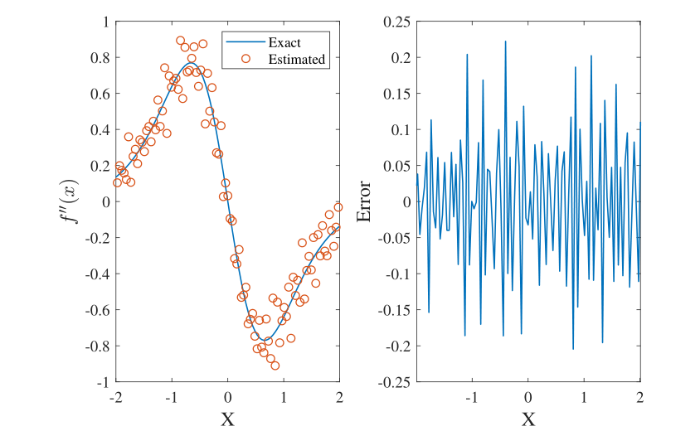
例 3.1 利用三阶 MQ 拟插值格式数值模拟函数的二阶导数. 考虑函数

f(x) = \tanh (x), - 2 \le x \le 2,

其二阶导数的精确解为

f"(x) = \frac{{8{{\rm e}^{ - x}}}}{{{{({{\rm e}^{ - x}} + {{\rm e}^x})}^3}}} - \frac{{8{{\rm e}^x}}}{{{{({{\rm e}^{ - x}} + {{\rm e}^x})}^3}}}.

选取 h = 0.04, \sigma = {h^3},K = 101. 由于随机性在研究中起到关键作用, 为了使实验结果可验证, 各方法均使用随机种子为 2023. MQ 函数的形状参数 c 对数值结果具有显著影响, 表 1 是不同形状参数 c 的敏感性分析, 由表 1 看出, c = 0.2{h^{1/5}} 是较优的选择, 这里均方误差 {E_2}、 最大误差 {E_\infty } 的计算公式如下所示

\begin{array}{l} {E_2} = \sqrt {\frac{1}{{{K^2}}}\sum\limits_{i = 0}^K {{{\left( {W({x_i},{y_j}) - \hat W({x_i},{y_j})} \right)}^2}} }, \\ {E_\infty } = \mathop {\max }\limits_{i,j} \left| {W({x_i},{y_j}) - \hat W({x_i},{y_j})} \right|. \end{array}

图 1图 2 分别表示, 在考虑随机误差的情况下, 三阶 MQ 拟插值算子和经典的有限差分法 [9] 对函数二阶导数的逼近效果. 左侧的图是逼近效果展示, 实线代表二阶导数的精确解, 圆点分别表示两种方法插值得到的高阶导数值. 右侧的图表示逼近误差, 即 f"(x) - \hat f"(x)f"(x) - \Delta \hat f"(x). 从图中可以看出, 基于三阶 MQ 拟插值方法得到的点与实线的距离更紧密, 受随机误差影响较小, 而且误差的波动范围更小, 对于高阶导数的逼近效果更好, 说明三阶 MQ 拟插值方法在解决该问题时具有更好的适用性.

表 1   三阶 MQ 形状参数 c 的敏感性分析

新窗口打开| 下载CSV


图1

图1   三阶 MQ 拟插值逼近二阶导数图像和误差


图2

图2   有限差分法逼近二阶导数图像和误差


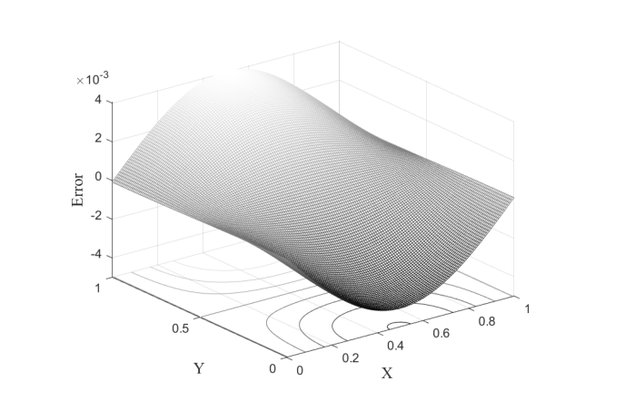
例3.2 利用三阶 MQ 拟插值计算拉普拉斯算子. 考虑如下函数

u(x,y) = \sin (\pi x) \cos(\pi y), \Omega = [0,1] \times [0,1],

其拉普拉斯算子为

{\nabla ^2}u(x,y) = - 2{\pi ^2}\sin (\pi x)\cos (\pi y).

单变量三阶 MQ 拟插值结构在求解二维算例时, 使用了张量积的处理技巧, 构造了 {\rm T} = \Gamma \otimes {\Gamma _2} + {\Gamma _2} \otimes \Gamma 形式来近似拉普拉斯算子 {\nabla ^2}u(x,y), 其中 \Gamma = ({\Phi _i}({x_j})){\Gamma _2} = ({\Phi _i}^{\prime \prime }({x_j})) \otimes 表示克罗内克积. 本例采用三种不同阶数的 MQ 拟插值方法求解二维函数拉普拉斯算子, 并使用 21 \times 2151 \times 51 等四种节点分布系统地评估各方法性能. 三种方法均取 h = \frac{1}{{K - 1}}\sigma = {h^9}S = 2023, 其中 S 表示随机种子数.

实验数据表 2 显示, 随着节点的增加, 估计误差显著减小, 计算时间则显著增加. 这一现象在使用的所有方法中均有体现. 不同阶数的 MQ 方法在相同节点下的表现有所不同. 一般而言, 较高阶数的 MQ 方法在误差方面表现更优, 但计算时间相对较长. 由图 3图 4 可以看出, 一阶 MQ 方法在区域边界处误差较大, 在这一点上三阶 MQ 表现较好.

表 2   拉普拉斯算子的后验估计

新窗口打开| 下载CSV


图3

图3   一阶 MQ 方法模拟拉普拉斯算子的误差分布


图4

图4   三阶 MQ 方法模拟拉普拉斯算子的误差分布


例3.3 利用三阶 MQ 拟插值计算拉普拉斯算子. 考虑如下函数

u(x,y,z) = \sin (\pi x)\sin (\pi y)\sin (\pi z)\begin{array}{*{20}{c}},&\Omega \end{array} = [0,1] \times [0,1] \times [0,1]

其拉普拉斯算子为

{\nabla ^2}u(x,y,z) = - 3{\pi ^2}\sin (\pi x)\sin (\pi y)\sin (\pi z).

图5

图5   三阶 MQ 方法模拟三维拉普拉斯算子的误差分布


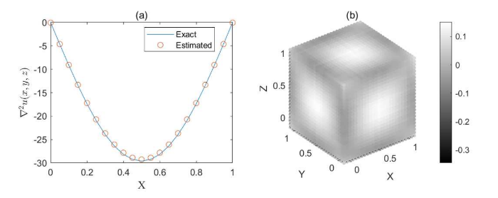
在例 2 的基础上扩展研究高维算例. 同样地, 使用张量积的处理办法构造了 {\rm T} = {\Gamma _2} \otimes \Gamma \otimes \Gamma + \Gamma \otimes {\Gamma _2} \otimes \Gamma + \Gamma \otimes \Gamma \otimes {\Gamma _2} 来近似算子. 选取 K = 21, h = \frac{1}{{K - 1}}, {\sigma = {h^5}}, S = 2023, c = 0.55{h^{1/5}}, 图 5(a) 是当 y=0.5,z=0.5 时, x 方向上的逼近情况, 图 5(b) 则通过颜色直观表达了误差的空间分布情况, 进一步验证了三阶 MQ 方法在高维问题中的适用性.

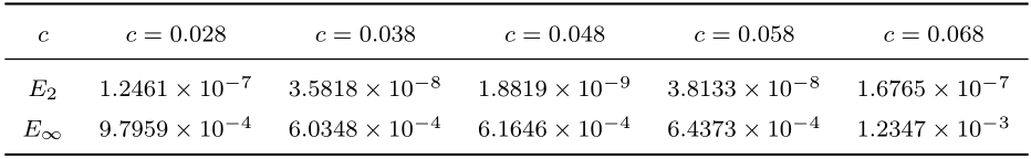
例3.4 利用三阶 MQ 拟插值方法求发展方程数值解. 考虑以下热方程

{u_t} = 2{u_{xx}}, 0 \le x \le 1,0 \le t \le 1,

边界条件为

\left\{ \begin{array}{l} u(x,0) = 2\cosh x,\qquad\qquad\, 0 \le x \le 1,\\ u(0,t) = 2{{\rm e}^{2t}},\qquad\qquad\qquad 0 \le t \le 1,\\ u(1,t) = ({e^2} + 1){{\rm e}^{2t - 1}},\quad\ \ \ 0 \le t \le 1, \end{array} \right.

可以证实该问题精确解为

u(x,t) = {{\rm e}^{2t + x}} + {{\rm e}^{2t - x}}.

在空间方向, 利用三阶 MQ 拟插值逼近空间导数, 在时间方向, 用向前差分法进行离散. 有限差分方法在时间和空间上则分别用中心差分与向前差分离散. 在时刻 t=1 时, 将 FDM 方法和三阶 MQ(Cubic MQ) 方法进行了精度比较, 计算结果如表 4 所示. 从逼近效果和误差精度的角度分析, 三阶 MQ 方法精度更高, 逼近效果更好. 表 4 中选取了 h = 0.1 \tau = 0.002\sigma = {h^3}S=2023, 其中 h 表示空间步长, \tau 表示时间步长. 并采用留一交叉验证法[4,6]确定了最优参数 c0.048, 从表 3 的敏感性分析中, 可以清晰观察到随着 c 值偏离最优值, 误差呈现逐渐增大的趋势.

表 3   形状参数 c 的敏感性分析

新窗口打开| 下载CSV


表 4   三阶 MQ 和 FDM 方法在 t=1 时的数值结果对比

新窗口打开| 下载CSV


参考文献

Beatson R K, Powell M J D.

Univariate multiquadric approximation: Quasi-interpolation to scattered data

Constructive Approximation, 1992, 8(3): 275-288

[本文引用: 2]

Buhmann M D.

Multivariate interpolation in odd-dimensional Euclidean spaces using multiquadrics

Constructive Approximation, 1990, 6(1): 21-34

[本文引用: 1]

Chen R H, Wu Z M.

Applying multiquadric quasi-interpolation to solve Burgers' equation

Applied Mathematics and Computation, 2006, 172(1): 472-484

[本文引用: 1]

Chen W, Fu Z J, Chen C S. Recent Advances in Radial Basis Function Collocation Methods. Berlin: Springer, 2014

[本文引用: 1]

Fasshauer G E.

Newton iteration with multiquadrics for the solution of nonlinear PDEs

Computers & Mathematics with Applications, 2002, 43(3-5): 423-438

[本文引用: 1]

Fasshauer G E, Zhang J G.

On choosing "optimal" shape parameters for RBF approximation

Numerical Algorithms, 2007, 45(1-4): 345-368

[本文引用: 1]

Franke R.

Scattered data interpolation: tests of some methods

Mathematics of Computation, 1982, 38(357): 181-200

[本文引用: 1]

Gao Q J, Wu Z M, Zhang S G.

Applying multiquadric quasi-interpolation for boundary detection

Computers & Mathematics with Applications, 2011, 62(12): 4356-4361

[本文引用: 1]

Godunov S K, Bohachevsky I.

Finite difference method for numerical computation of discontinuous solutions of the equations of fluid dynamics

Matematičeskij Sbornik, 1959, 47(3): 271-306

[本文引用: 1]

Hardy R L.

Multiquadric equations of topography and other irregular surfaces

Journal of Geophysical Research, 1971, 76(8): 1905-1915

[本文引用: 1]

Hon Y C, Mao X Z.

An efficient numerical scheme for Burgers' equation

Applied Mathematics and Computation, 1998, 95(1): 37-50

[本文引用: 1]

Ma L M, Wu Z M.

Approximation to the k-th derivatives by multiquadric quasi-interpolation method

Journal of Computational and Applied Mathematics, 2009, 231(2): 925-932

[本文引用: 1]

Ma L M, Wu Z M.

Stability of multiquadric quasi-interpolation to approximate high order derivatives

Science China Mathematics, 2010, 53(4): 985-992

[本文引用: 3]

Mittal R C, Tripathi A.

Numerical solutions of generalized Burgers-Fisher and generalized Burgers-Huxley equations using collocation of cubic B-splines

Int J Comput Math, 2015, 92(5): 1053-1077

[本文引用: 1]

Wu Z M, Schaback R.

Shape preserving properties and convergence of univariate multiquadric quasi-interpolation

Acta Mathematicae Applicatae Sinica, 1994, 10(4): 441-446

[本文引用: 2]

Wu Z M, Zhang S L.

Conservative multiquadric quasi-interpolation method for Hamiltonian wave equations

Engineering Analysis with Boundary Elements, 2013, 37(7/8): 1052-1058

[本文引用: 1]

Zhang S L, Yang H Q, Yang Y.

A multiquadric quasi-interpolations method for CEV option pricing model

Journal of Computational and Applied Mathematics, 2019, 347: 1-11

DOI:10.1016/j.cam.2018.03.046      [本文引用: 1]

The pricing of option contracts when the underlying process follows the constant elasticity of variance (CEV) model is considered. For CEV European options, the closed-form solutions involve the non-central chi-square distribution, whose computations by the current literatures are rather unstable and extremely expensive. Based on multiquadric quasi-interpolation methods, this study suggests a stable and fast numerical algorithm for CEV option pricing model. The method is confirmed to be a multinomial tree, in which the underlying variable moves from its initial value to an infinity of possible values of the next time step. The probabilities in the associated tree are ensured to be positive, which is a sufficient condition for stability and convergence. The method is flexible, since it is simple to implement with the nonuniform knots. Moreover, the method is easy to value the Greek letters which are important parameters in financial engineering, as the multiquadric function is infinitely continuously differentiable. Besides, the method does not require solving a resultant full matrix, the ill-conditioning problem arising when using the radial basis functions as a global interpolant can be avoided. Numerical experiments imply that the method is highly effective to calculate the stock options and its Greeks under the CEV model. (C) 2018 Elsevier B.V.

Zhu C G, Kang W S.

Numerical solution of Burgers-Fisher equation by cubic B-spline quasi-interpolation

Applied Mathematics and Computation, 2010, 216(9): 2679-2686

[本文引用: 1]

/