

1 模型与问题
在众多性传播疾病中, 梅毒的流行范围很广, 对患者的身心健康构成严重威胁. 在青霉素出现之前, 梅毒是一种重要的致命和致残疾病. 在医学史上, 梅毒、结核病和麻风病被列为世界三大慢性病[1]. 梅毒发病率在 20 世纪 80 年代和 90 年代有所下降, 部分原因是艾滋病病毒开始流行, 以及各国对安全性行为的大量科学宣传. 然而, 自 21 世纪初以来, 梅毒的发病率急剧上升, 在一些国家激增了 300%[2]. 根据中国疾病预防控制中心的数据, 2020 年中国新增梅毒病例 464345 例. 来自东京传染病信息中心的数据显示, 2020 年日本累计确诊梅毒病例超过 1 万例, 达到 10141 例[3]. 梅毒的预防和科学研究涉及预防医学、临床医学和传染病动力学. 因此, 梅毒的动力学建模和研究已成为生物数学的一个重要分支, 控制梅毒的流行对保障人们的身心健康具有重要意义.
在文献 [4,5] 的经典梅毒建模工作基础上, 很多研究者提出了许多数学模型来研究梅毒疾病的传播动力学, 这里我们详细地讨论了与当前论文中开展的工作相关的一些值得注意的工作. Grassly 等人[6] 利用美国疾病控制与预防中心 1941 年至 2002 年间对美国 68 个城市的数据, 将真实数据应用于 SIRS 梅毒模型. Iboi 和 Okuonghae[7] 研究了梅毒数学模型的群体动力学, 他们的工作表明, 初级和次级阶段梅毒感染者的高治疗率对感染剩余阶段的梅毒感染者群体有积极影响. Saad-Roy 等人[8] 建立了数学模型来研究传播 MSM 人群中梅毒的传播动力学, 他们的工作量化了早期治疗对梅毒控制的重要性. Gumel 等人[9] 提出了一个新的两组性别结构模型, 用于评估治疗和避孕套使用对梅毒传播动力学和控制的社区层面影响. Nwankwo 和 Okuonghae[10] 建立了一个数学模型以研究在梅毒治疗的情况下 HIV-梅毒联合感染的动力学行为. Omame 等人[11] 建立了 HPV 和梅毒的共同感染模型并研究了该模型的最佳控制和成本效益分析. 此外, 基于梅毒感染机制, 已有研究者建立了诸多数学模型来研究梅毒的传播以及不同地区的治疗、避孕套使用、异质性严重程度和封锁对梅毒传播的影响. 然而, 就我们所见, 这些工作主要基于常微分方程 (ODEs) 来研究梅毒在人群中的传播. 从传染病角度出发, 在疾病传播中空间因素通常是不容忽视[12,13]. 事实上, 梅毒的传播表现出明显的空间扩散特征. 虽然一些结果已表明空间异质性对梅毒在中国的传播有明显影响, 但通过数学模型对异质环境中空间扩散对梅毒的影响研究很少. 由鉴于此, 在文献 [7] 的基础上, 本文将人群分为以下 6 个仓室: 易感人群 (
模型 (1.1) 具有如下初边值条件
其中
为了后续对系统 (1.1) 进行动力学分析, 首先我们从生物学角度出发对模型参数给出如下假设
假设 1.1 对于系统 (1.1), 假设
(A1) 函数
(A2) 函数
(A3) 扩散率
接下来讨论模型 (1.1) 的适定性问题. 首先考虑下列抛物型系统
由假设 1.1 (A1) 以及引理 3.2[14] 可得如下结论
引理 1.1 系统 (1.2) 存在唯一的正平衡态
令空间
令
引理 1.2 如果系统 (1.1) 具有初值条件
定理 1.1 对于具有初值条件
证 令
显然系统 (1.3) 的特征值问题存在一个具有强正特征函数
根据常微分方程比较原理可知存在
这意味着
定理 1.1 结论表明系统 (1.1) 的解半流
定理 1.2 系统 (1.1) 的解半流
2 系统 (1.1) 基本再生数及阈值动力学
此节中, 我们致力于推导模型 (1.1) 的基本再生数泛函表达式并研究系统 (1.1) 的阈值动力学行为. 由引理1.1 可知系统 (1.1) 总存在唯一的无病平衡态
显然系统 (2.1) 是合作系统. 因而系统 (2.1) 有唯一的具有强正特征函数
则新增感染个体总数量为
根据下一代再生算子的定义可知系统 (1.1) 的基本再生数
引理 2.1 系统 (2.1) 的主特征值
定理 2.1 如果
证 根据抛物型方程的比较原理可知当
假设
其中
这意味着
从而可得
现在证明系统 (1.1) 的一致持久性. 为此, 给出下列记号
定理 2.2 对于具有初值条件
此外, 系统 (1.1) 至少存在一个正平衡态.
证 我们分三步证明. 第一步, 证明
令
定理 2.3 假设系统 (1.1) 除了扩散系数
证 由定理 2.1 可知系统 (1.1) 在
定义李雅普诺夫函数
其中
令
注意到
显然对
3 数值模拟
此节, 我们对系统 (1.1) 进行数值模拟. 为了方便起见, 假设空间
3.1 系统 (1.1) 解的动力学行为刻画
根据式 (3.1) 中列出的参数值, 利用文献 [21] 中的计算方法可估算出模型 (1.1) 基本再生数
图1
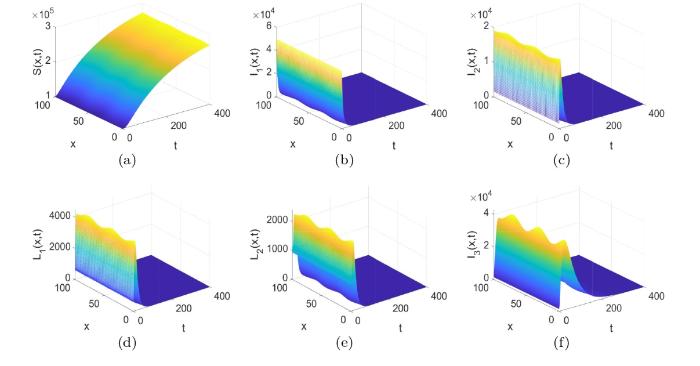
图2
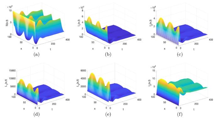
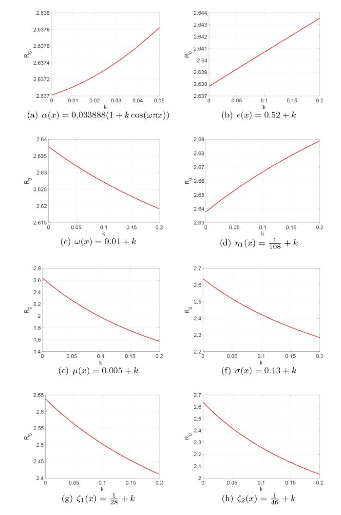
图3
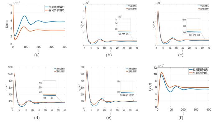
3.2 空间异质性对梅毒传播的影响
此小节, 为了研究空间异质性对梅毒传播的影响, 我们在空间同质和空间异质两种情形下进行数值模拟并作出比较说明. 首先我们记
图4
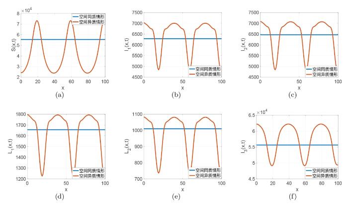
图5
3.3 初值和扩散系数 d_i(x) 对梅毒传播的影响
此小节我们分析初值条件和扩散率
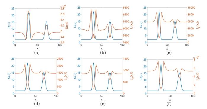
为了研究扩散率 d_i(x) 没梅毒传播的影响, 令 \alpha(x)=\tilde{\alpha},\beta(x)=\tilde{\beta},\gamma(x)=\tilde{\gamma} 以及 d_i(x)=d_iD(x), D(x)=2+\frac{50}{\sqrt{2\pi }}\exp\left(-\frac{(x-30)^2}{8}\right)+\frac{100}{3\sqrt{2\pi }}\exp\left(-\frac{(x-70)^2}{18}\right),x\in[0,100],i=1,2,3,4,5,6, 这里的 D(x) 是包含两个 Gaussia 类型的扩散率函数. 其他参数同式 (3.1).
图6 和 7 分别对应初值条件 (3.2) 和 (3.3) 解的演化行为. 从这两个图中我们可以看出初值的分布不会影响系统 (1.1) 解的最终演化趋势, 这说明初值几乎不影响梅毒在长时间内的传播趋势. 图8 刻画的是 Gaussia 类型扩散率函数
图6
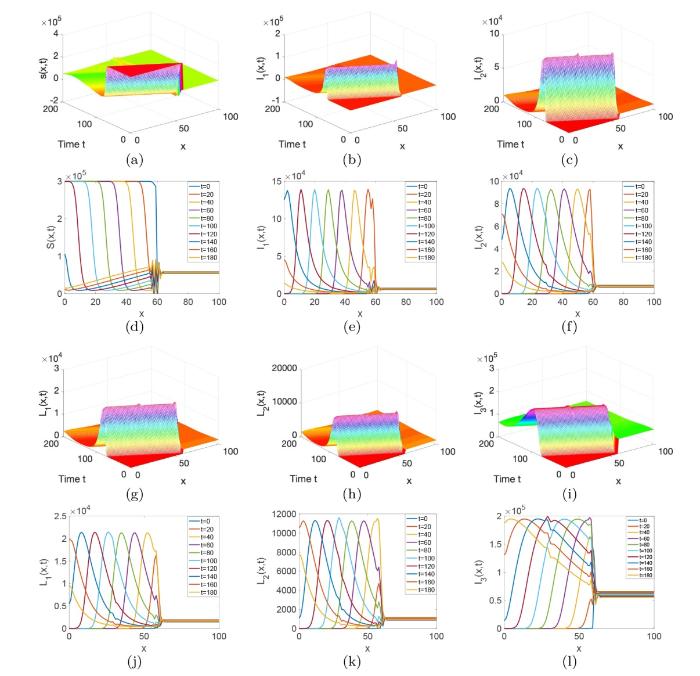
图6
系统 (1.1) 在初值条件 (3.2) 下解的演化行为,
图7
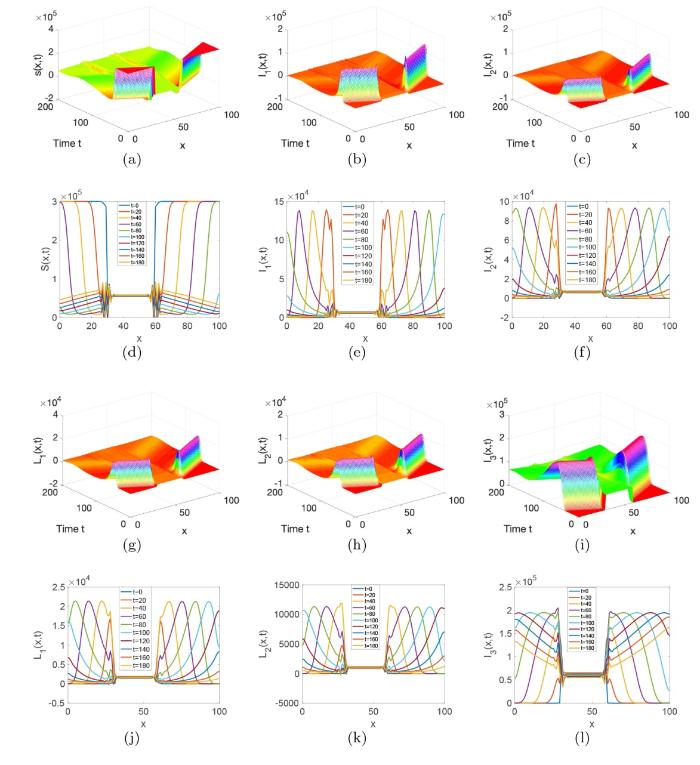
图7
系统 (1.1) 在初值条件 (3.3) 下解的演化行为,
图8
4 结论
本文构建了一类具有异质空间反应扩散梅毒动力学模型去研究个体扩散和空间异质环境对梅毒传播的影响. 理论分析部分, 我们首先讨论了解的全局存在性、系统的耗散性和解半流吸引子存在性; 利用下一代再生算子定义推导出模型的基本再生数
参考文献
Global phylogeny of Treponema pallidum lineages reveals recent expansion and spread of contemporary syphilis
DOI:10.1038/s41564-021-01000-z
PMID:34819643
[本文引用: 1]

Syphilis, which is caused by the sexually transmitted bacterium Treponema pallidum subsp. pallidum, has an estimated 6.3 million cases worldwide per annum. In the past ten years, the incidence of syphilis has increased by more than 150% in some high-income countries, but the evolution and epidemiology of the epidemic are poorly understood. To characterize the global population structure of T. pallidum, we assembled a geographically and temporally diverse collection of 726 genomes from 626 clinical and 100 laboratory samples collected in 23 countries. We applied phylogenetic analyses and clustering, and found that the global syphilis population comprises just two deeply branching lineages, Nichols and SS14. Both lineages are currently circulating in 12 of the 23 countries sampled. We subdivided T. p. pallidum into 17 distinct sublineages to provide further phylodynamic resolution. Importantly, two Nichols sublineages have expanded clonally across 9 countries contemporaneously with SS14. Moreover, pairwise genome analyses revealed examples of isolates collected within the last 20 years from 14 different countries that had genetically identical core genomes, which might indicate frequent exchange through international transmission. It is striking that most samples collected before 1983 are phylogenetically distinct from more recently isolated sublineages. Using Bayesian temporal analysis, we detected a population bottleneck occurring during the late 1990s, followed by rapid population expansion in the 2000s that was driven by the dominant T. pallidum sublineages circulating today. This expansion may be linked to changing epidemiology, immune evasion or fitness under antimicrobial selection pressure, since many of the contemporary syphilis lineages we have characterized are resistant to macrolides.© 2021. The Author(s).
The natural history of syphilis: Implications for the transmission dynamics and control of infection
Infectious syphilis in high-income settings in the 21st century
DOI:10.1016/S1473-3099(08)70065-3
PMID:18353265
[本文引用: 1]
In high-income countries after World War II, the widespread availability of effective antimicrobial therapy, combined with expanded screening, diagnosis, and treatment programmes, resulted in a substantial decline in the incidence of syphilis. However, by the turn of the 21st century, outbreaks of syphilis began to occur in different subpopulations, especially in communities of men who have sex with men. The reasons for these outbreaks include changing sexual and social norms, interactions with increasingly prevalent HIV infection, substance abuse, global travel and migration, and underinvestment in public-health services. Recently, it has been suggested that these outbreaks could be the result of an interaction of the pathogen with natural immunity, and that syphilis epidemics should be expected to intrinsically cycle. We discuss this hypothesis by examining long-term data sets of syphilis. Today, syphilis in western Europe and the USA is characterised by low-level endemicity with concentration among population subgroups with high rates of partner change, poor access to health services, social marginalisation, or low socioeconomic status.
Host immunity and synchronized epidemics of syphilis across the United States
Population dynamics of a mathematical model for syphilis
A mathematical model of syphilis transmission in an MSM population
DOI:10.1016/j.mbs.2016.03.017
PMID:27071977
[本文引用: 1]
Syphilis is caused by the bacterium Treponema pallidum subspecies pallidum, and is a sexually transmitted disease with multiple stages. A model of transmission of syphilis in an MSM population (there has recently been a resurgence of syphilis in such populations) that includes infection stages and treatment is formulated as a system of ordinary differential equations. The control reproduction number is calculated, and it is proved that if this threshold parameter is below one, syphilis dies out; otherwise, if it is greater than one, it is shown that there exists a unique endemic equilibrium and that for certain special cases, this equilibrium is globally asymptotically stable. Using data from the literature on MSM populations, numerical methods are used to determine the variation and robustness of the control reproduction number with respect to the model parameters, and to determine adequate treatment rates for syphilis eradication. By assuming a closed population and no return to susceptibility, an epidemic model is obtained. Final outbreak sizes are numerically determined for various parameter values, and its variation and robustness to parameter value changes is also investigated. Results quantify the importance of early treatment for syphilis control.Copyright © 2016 Elsevier Inc. All rights reserved.
Mathematics of a sex-structured model for syphilis transmission dynamics
Mathematical analysis of the transmission dynamics of HIV syphilis co-infection in the presence of treatment for syphilis
A co-infection model for HPV and syphilis with optimal control and cost-effectiveness analysis
基于空间异质反应扩散 HIV 感染模型的最优治疗策略
本文研究一类空间异质反应扩散HIV感染模型的最优治疗问题.借助最小化序列技巧确立了最优策略的存在性.随后,通过应用凸摄动理论给出最优控制满足的一阶必要条件.在不考虑末端时刻控制成本的情况下给出了Bang-Bang形式的最优策略.数值模拟验证了同时采取三个治疗策略能够显著降低 HIV病毒以及感染细胞的载量从而有效地控制HIV在宿主体内的感染进程.
Optimal treatment strategies for a reaction-dffusion HIV infection model with spatial heterogeneity
本文研究一类空间异质反应扩散HIV感染模型的最优治疗问题.借助最小化序列技巧确立了最优策略的存在性.随后,通过应用凸摄动理论给出最优控制满足的一阶必要条件.在不考虑末端时刻控制成本的情况下给出了Bang-Bang形式的最优策略.数值模拟验证了同时采取三个治疗策略能够显著降低 HIV病毒以及感染细胞的载量从而有效地控制HIV在宿主体内的感染进程.
Modeling rabies transmission in spatially heterogeneous environments via
Threshold dynamics of a delayed nonlocal reaction-diffusion HIV infection model with both cell-free and cell-to-cell transmissions
Abstract functional differential equations and reaction-diffusion systems
Semigroups of Linear Operators and Applications to Partial Differential Equations
A reaction-diffusion within-host HIV model with cell-to-cell transmission
DOI:10.1007/s00285-017-1202-x
PMID:29305736
[本文引用: 2]
In this paper, a reaction-diffusion within-host HIV model is proposed. It incorporates cell mobility, spatial heterogeneity and cell-to-cell transmission, which depends on the diffusion ability of the infected cells. In the case of a bounded domain, the basic reproduction number [Formula: see text] is established and shown as a threshold: the virus-free steady state is globally asymptotically stable if [Formula: see text] and the virus is uniformly persistent if [Formula: see text]. The explicit formula for [Formula: see text] and the global asymptotic stability of the constant positive steady state are obtained for the case of homogeneous space. In the case of an unbounded domain and [Formula: see text], the existence of the traveling wave solutions is proved and the minimum wave speed [Formula: see text] is obtained, providing the mobility of infected cells does not exceed that of the virus. These results are obtained by using Schauder fixed point theorem, limiting argument, LaSalle's invariance principle and one-side Laplace transform. It is found that the asymptotic spreading speed may be larger than the minimum wave speed via numerical simulations. However, our simulations show that it is possible either to underestimate or overestimate the spread risk [Formula: see text] if the spatial averaged system is used rather than one that is spatially explicit. The spread risk may also be overestimated if we ignore the mobility of the cells. It turns out that the minimum wave speed could be either underestimated or overestimated as long as the mobility of infected cells is ignored.
