PNP 方程的基于高斯过程回归的新 Gummel 迭代算法

PNP 方程的基于高斯过程回归的新 Gummel 迭代算法

敖渝焱, 阳莺^,^*

桂林电子科技大学数学与计算科学学院 & 广西应用数学中心 (GUET) & 广西高校数据分析与计算重点实验室广西桂林 541004

A New Gummel Iterative Algorithm Based on Gaussian Process Regression for the PNP Equation

Ao Yuyan, Yang Ying^,^*

Guilin University of Electronic Technology, School of Mathematics and Computating Science & Guangxi Applied Mathematics Center (GUET) & Guangxi Colleges and Universities Key Laboratory of Data Analysis and Computation, Guangxi Guilin 541004

通讯作者: *阳莺, E-mail: yangying@lsec.cc.ac.cn

收稿日期: 2023-12-13 修回日期: 2024-04-15

基金资助:

国家自然科学基金(12161026)
广西科技基地和人才专项(AD23026048)
广西自然科学基金(2020GXNSFAA159098)
广西科技项目(AD23023002)

Received: 2023-12-13 Revised: 2024-04-15

Fund supported:

NSFC(12161026)
Special Fund for Scientific and Technological Bases and Talents of Guangxi(AD23026048)
Guangxi Natural Science Foundation(2020GXNSFAA159098)
Science and Technology Project of Guangxi(AD23023002)

摘要

Poisson-Nernst-Planck (PNP) 方程是由 Poisson 方程和 Nernst-Planck 方程耦合而成的一类非线性偏微分方程组, 其常用的线性化迭代方法-Gummel 迭代的效率很大程度上受松弛参数的影响. 机器学习中的高斯过程回归 (GPR) 方法因其训练规模较小, 且不需要提供函数关系, 在该文中被应用于预测 Gummel 迭代的较优松弛参数, 加速迭代的收敛速度. 首先针对 PNP 方程的 Gummel 迭代, 设计了一种可预测松弛参数的 GPR 方法. 其次利用 Box-Cox 转换方法, 对 Gummel 迭代的数据进行预处理, 提高 GPR 方法的准确性. 最后基于 GPR 方法及 Box-Cox 转换算法, 提出了 PNP 方程的一种新的 Gummel 迭代算法. 数值实验表明, 新 Gummel 迭代算法与经典的 Gummel 迭代算法相比, 求解效率更高, 且收敛阶相同.

关键词： Poisson-Nernst-Planck 方程; Gummel 迭代; 高斯过程回归; 参数预测; 机器学习

Abstract

PNP Equations are a class of nonlinear partial differential equations coupled from Poisson and Nernst planck equations, and the efficiency of its Gummel iteration, a commonly used linearization iteration method, is largely affected by the relaxation parameter. The Gaussian Process Regression (GPR) method in machine learning, due to its small training size and the fact that it does not need to provide a functional relationship, is applied in that paper to predict the preferred relaxation parameters for the Gummel iteration and accelerate the convergence of the iteration. Firstly GPR method with predictable relaxation parameters is designed for the Gummel iteration of the PNP equation. Secondly, the Box-Cox transformation method is utilized to preprocess the data of Gummel iteration to improve the accuracy of the GPR method. Finally, based on the GPR method and Box-Cox transformation algorithm, a new Gummel iteration algorithm for the PNP equation is proposed. Numerical experiments show that the new Gummel iterative algorithm is more efficient in solving and has the same convergence order compared to the classical Gummel iterative algorithm.

Keywords： Poisson-Nernst-Planck equations; Gummel iteration; Gaussian process regression; Parameter prediction; Machine learning

PDF (614KB) 元数据多维度评价相关文章导出 EndNote| Ris| Bibtex 收藏本文

本文引用格式

敖渝焱, 阳莺. PNP 方程的基于高斯过程回归的新 Gummel 迭代算法[J]. 数学物理学报, 2024, 44(5): 1301-1309

Ao Yuyan, Yang Ying. A New Gummel Iterative Algorithm Based on Gaussian Process Regression for the PNP Equation[J]. Acta Mathematica Scientia, 2024, 44(5): 1301-1309

1 引言

Poisson-Nernst-Planck 方程, 简称为 PNP 方程, 可用来描述生物分子系统的电扩散反应过程, 并且该模型已经被广泛的应用于电化学、半导体、生物膜通道等领域^[1]. 由于 PNP 方程是一个非线性的耦合系统, 常需要利用解耦方法进行求解, 而 Gummel 迭代是一种广泛应用于求解 PNP 方程的解耦方法. 对于实际 PNP 问题, 通常需要利用松弛参数才能保证 Gummel 迭代收敛. 而松弛参数的取值对 Gummel 迭代的收敛效果影响较大, 传统的 Gummel 迭代法都是按照经验来给定松弛参数取值, 然而, 按照经验取值一般不是较优松弛参数, 可能造成 PNP 方程迭代时间很长, 迭代速度很慢.

近年来机器学习技术被引入到各种模型的数值计算中, 通过预测出较优参数, 来加速数值解的收敛, 降低数值模拟中的计算成本. 比如 Mukerji 等人^[2] 利用随机森林回归加速多相多孔介质流的求解. Jiang 等人^[3] 引入了高斯过程回归 (GPR) 来预测交替方向隐式方法 (ADI) 中的参数, 以提高求解的效率和准确性. Uyan^[4] 使用机器学习方法来预测水下传感器网络参数, 提高水下传感器网络的性能和可靠性. Sudhir^[5] 使用人工神经网络 (ANN) 和递归神经网络 (RNN) 模型来预测车轮接触参数, 来减少脱轨倾向、车轮磨损和能耗. 我们注意到最近也出现了少量利用机器学习方法求解 PNP 方程的工作, 如文献 [6] 利用接口神经网络方法 (INNs) 求解 PNP 方程, 加速方程收敛和提高数值精度. 但是该文主要侧重于利用机器学习算法求解, 而不是用于预测参数. 据我们所知, 目前还没有利用机器学习来预测 PNP 方程迭代算法参数的相关工作. 本文针对一类 PNP 方程, 利用 GPR 方法对 Gummel 迭代的松弛参数进行预测, 得到较优参数, 提高 Gummel 迭代的收敛效率. 首先, 针对 PNP 方程的 Gummel 迭代设计了 GPR 方法. 其次, 利用 Box-Cox 转换算法, 对 GPR 的训练集进行处理, 使其接近高斯分布, 提高 GPR 方法的准确性. 然后基于 GPR 方法及 Box-Cox 转换算法给出一种新的 Gummel 算法. 数值实验表明: 这一新算法与经典的 Gummel 算法相比, 在收敛阶相同的情况下, 计算效率更高.

2 PNP 方程及有限元离散

本文考虑一种在半导体领域中的 PNP 方程^[7]

$\begin{align*} & -\nabla\cdot\nabla u=\frac{e_c^2\beta}{\varepsilon_0\varepsilon_s}(p-n), \mbox{在}\ \Omega\ \mbox{内,} \end{align*}$

(2.1)

$\begin{align*} & -\nabla\cdot D_p(\nabla p+p\nabla u)=f_p, \mbox{在}\ \Omega\ \mbox{内,} \end{align*}$

(2.2)

$\begin{align*} &-\nabla\cdot D_n(\nabla n-n\nabla u)=f_n, \mbox{在}\ \Omega\ \mbox{内,} \end{align*}$

(2.3)

其中静电势 $u$ , 空穴浓度 $p$ , 电子浓度 $n$ 是方程的未知量, 区域的相对介电常数用 $\varepsilon_s$ 表示, 真空介电常数用 $\varepsilon_0$ 表示, $e_c$ 为单位电荷量, $\beta=\frac{1}{k_{\mathrm{B}}T}$ 为 Boltzmann 能量的倒数, $k_B$ 为 Boltzmann 常数, T 为开尔文温度, $D_p$ 和 $D_n$ 分别为空穴和电子的扩散系数. 其边界条件为 Dirichlet 边界条件

$\begin{equation}\label{} u|_{\partial\Omega}=u_d, p|_{\partial\Omega}=p_d, n|_{\partial\Omega}=n_d. \end{equation}$

(2.4)

其中, $u_d$ , $p_d$ , $n_d$ 为已知函数. 方程 (2.1) 为 Possion 方程, 在半导体领域内也称电势方程, 可以描述半导体器件中的电势分布情况, 进而了解到载流子浓度分布、电场和电势梯度等相关量. 方程 (2.2)-(2.3) 为 NP 方程, 描述空穴和电子两种载流子的运动规律, 又称为载流子连续性方程.

2.1 弱形式及有限元离散

设 $\Omega$ 是 $\mathbb{R}^{3}$ 中的有界区域, 满足 Lipchitz 连续, $\partial\Omega$ 表示边界. $H^1(\Omega)$ 表示自身及一阶导数属于 $L^2(\Omega)$ 的函数构成的 Sobolev 空间, $C^0(\Omega)$ 表示区域上的连续函数空间, 定义 $H_{0}^{1}(\Omega)=\left\{v \in H^{1}(\Omega):\left.v\right|_{\partial \Omega}=0\right\}$ , $(\cdot,\cdot)$ 表示 $L^2_{\Omega}$ 内积, 满足 $(u,v)=\int_{\Omega} u(x) v(x){\rm d}x,$ 定义

$V_p=\left\{v\in H^1(\Omega):v|_{\partial\Omega}=p_d\right\}, V_n=\left\{v\in H^1(\Omega):v|_{\partial\Omega}=n_d\right\},$

$V_u=\left\{u\in H^1(\Omega):u|_{\partial\Omega}=u_d\right\}.$

则方程 (2.1)-(2.3) 的变分形式为: 寻找 $p\in V_p, n\in V_n, u\in V_u$ , 满足以下方程

$\begin{align*}\label{1.6} &D_p(\nabla p, \nabla v)+D_p(\nabla p \nabla u, \nabla v)=\left(f_{p}, v\right), \forall v \in H_{0}^{1}(\Omega),\\ &D_n(\nabla n, \nabla v)+D_n(\nabla n \nabla u, \nabla v)=\left(f_{n}, v\right), \forall v \in H_{0}^{1}(\Omega),\\ &-(\nabla {u},\nabla w)=\bigg(\frac{e_c^2\beta}{\varepsilon_0\varepsilon_s}(p-n),w\bigg), \forall w \in H_{0}^{1}(\Omega). \end{align*}$

(2.5)

区域 $\Omega$ 的一个有限划分 $\Gamma_h$ 是一个单元集合 $\left \{ e \right \}$ , $e$ 是剖分单元, 对每一单元 $e\in \Gamma_h$ , $P^{\mathrm{l}}(e)$ 表示线性多项式的集合. 定义如下线性有限元空间

$\begin{align*} &\left.S^{h}_p=\left\{\nu\subset H^{1}(\Omega):\nu\right|_{e}\in P^{1}(e),\:\forall e\in \Gamma_{h}(\Omega), v|_{\partial\Omega}=p_d\right\}, \\ &\left.S^{h}_n=\left\{\nu\subset H^{1}(\Omega):\nu\right|_{e}\in P^{1}(e),\:\forall e\in \Gamma_{h}(\Omega), v|_{\partial\Omega}=n_d\right\}, \\ & \left.S^{h}_u=\left\{\nu\subset H^{1}(\Omega):\nu\right|_{e}\in P^{1}(e),\:\forall e\in \Gamma_{h}(\Omega), v|_{\partial\Omega}=u_d\right\}, \\ & \left.S_{0}^{h}=\left\{\nu\subset H^{1}(\Omega):\nu\right|_{e}\in P^{1}(e),\:\forall e\in T_{h}(\Omega), v|_{\partial\Omega}=0\right\}. \end{align*}$

其中, 方程 (2.1)-(2.3) 的标准有限元离散如下寻找 $p_{h}\in S^{h}_p, n_{h}\in S^{h}_n, u_{h}\in S^{h}_u$ , 使得

$\begin{align*}\label{1.7} & D_p(\nabla p_{h}, \nabla v_{h})+D_p(\nabla p_{h}\nabla u_{h}, \nabla v_{h})=(f_{p}, v_{h}), \forall v_{h} \in S_{0}^{h}, \\ & D_n(\nabla n_{h}, \nabla v_{h})+D_n(\nabla n_{h}\nabla u_{h}, \nabla v_{h})=(f_{n},v_{h}), \forall v_{h} \in S_{0}^{h}, \\ & (\nabla u_h, \nabla w_h)=\bigg(\frac{e_c^2\beta}{\varepsilon_0\varepsilon_s}(p-n), w_h\bigg), \forall w_{h} \in S_{0}^{h}. \end{align*}$

(2.6)

2.2 Gummel 迭代

PNP 方程是一个强耦合、强非线性的偏微分方程组, 仅在极少数情形下能找到它的解析解. 由于 PNP 方程由两个以上的偏微分方程组成, 一般来说, 在大规模问题的应用中, 使用解耦方法求解比直接求解更方便, 并且数值实现更容易和高效. 目前用于求解 PNP 方程的主要解耦方法是 Gummel 迭代. Gummel 迭代不仅具有快速求解、较好的收敛性和稳定性, 而且可以根据实际需求灵活地调整迭代次数和收敛准则, 以达到所需的数值解精度, 其具体过程见算法 1.

算法 1 中的 $\alpha$ 就是 Gummel 迭代的松弛参数, 通常根据经验取值, 但是该参数的取值对 Gummel 迭代的迭代次数有着较大影响, 取值不合适, 迭代时间会很长, 浪费大量的计算成本. 考虑到机器学习方法可以根据数据的特征和模式来自动调整参数, 从而提高预测的准确性. 本文使用机器学习中的高斯过程回归算法, 选取出一个较优的松弛参数, 来加速 Gummel 迭代.

3 高斯过程回归

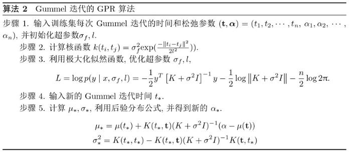
本节, 首先参考文献 [9] 的工作设计了针对 PNP 方程的 Gummel 迭代的 GPR 算法. 然后利用 Box-Cox 转换方法, 对 GPR 的训练集进行预处理. 最后我们给出基于 GPR 方法的新 Gummel 迭代算法.

3.1 PNP 方程 Gummel 迭代的 GPR 算法

高斯过程是指多变量高斯随机变量到无限 (可数或连续) 指数集的自然推广. GPR 是一种灵活的非参数回归方法, 对数据的分布假设较少, 它可以适应各种形式的数据, 并且在没有明确的函数形式假设下进行建模.

设有一组训练集 $D=(\textbf{t},\boldsymbol{\alpha})$ , 其中 $\textbf{t}=(t_1,t_2,\cdots,t_n)$ , 是指每次 Gummel 迭代的时间, $\boldsymbol{\alpha}=(\alpha_1,\alpha_2,\cdots,\alpha_n)$ 则对应 Gummel 迭代的松弛参数. $(\textbf{t},\boldsymbol{\alpha})$ 是一对输入输出. 假设对应于任何输入样本 $\textbf{t}$ , 对应的输出样本 $\boldsymbol{\alpha}$ 服从一个多元高斯分布, 则 $f(t)=[f(t_1),f(t_2),\cdots,f(t_n)]$ 也符合n维高斯分布, 即

$\left[\begin{array}{c}f\left(t_{1}\right) \\\vdots \\f\left(t_{n}\right)\end{array}\right] \sim N\left(\left[\begin{array}{c}\mu\left(t_{1}\right) \\\vdots \\\mu\left(t_{n}\right)\end{array}\right],\left[\begin{array}{ccc}k\left(t_{1}, t_{1}\right) & \cdots & k\left(t_{1}, t_{n}\right) \\\vdots & \ddots & \vdots \\k\left(t_{n}, t_{1}\right) & \cdots & k\left(t_{n}, t_{n}\right)\end{array}\right]\right).$

其中 $\mu$ 为均值函数, $k(t, t)$ 是核函数 (也称为协方差函数). 故上述过程可重写为 $f(t)\sim GP(\mu(t),k(t,t^{'})),$ 其中 $t$ , $t^{'}$ 是训练集 $\textbf{t}$ 中的任意两个变量. GPR 方法的任务是学习输入集 $\textbf{t}$ 和输出集 $\boldsymbol{\alpha}$ 之间的映射关系, 并在给定新的测试点 $t_*$ 的情况下推断出最可能的输出值, 在实际问题中, 设 $\boldsymbol{\alpha}=f(\textbf{t})+\varepsilon$ . $\varepsilon$ 是噪声来提高回归模型的泛化能力, 使其在面对新输入的数据时更具鲁棒性, $\varepsilon$ 符合高斯分布即 $\varepsilon \sim N(0,\sigma)$ , 故 $\boldsymbol{\alpha}=f(\textbf{t})+\varepsilon\sim N(\mu(\textbf{t}), k(t_{i},t_{j})+\sigma^{2}I).$

给定新的输入样本 $t_*$ , 我们希望预测相应的输出样本 $\alpha_*$ . 根据高斯过程的性质, 我们可以得到联合分布

$\begin{bmatrix}\alpha\\\alpha_*\end{bmatrix}\sim N\Bigg(\begin{bmatrix}\mu(t)\\\mu(t_*)\end{bmatrix},\begin{bmatrix}K+\sigma^2I&K(t,t_*)\\K(t_*,t)&K(t_*,t_*)\end{bmatrix}\Bigg),$

其中协方差矩阵 $K$ 表示为

$K=\begin{bmatrix} {k(t_{1},t_{1})}&{k(t_{1},t_{2})}&{\ldots}&{k(t_{1},t_{n})}\\{k(t_{2},t_{1})}&{k(t_{2},t_{2})}&{\ldots}&{k(t_{2},t_{n})}\\{\ldots}\\{k(t_{n},t_{1})}&{k(t_{n},t_{2})}&{\ldots}&{k(t_{n},t_{n})}\\ \end{bmatrix}.$

列向量和行向量 $K(\textbf{t},t_*)$ , $K(t_*,\textbf{t})$ 分别为

$K(\textbf{t},t_*)=[k(t_1,t_*),k(t_2,t_*),\cdots,k(t_n,t_*)]^T,$

$K(t_*,\textbf{t})=[k(t_1,t_*),k(t_2,t_*),\cdots,k(t_n,t_*)].$

在这里核函数 $k(t_i, t_j)$ 取指数核函数, 即

$k(t_{i},t_{j})=\sigma_{f}^{2}\mathrm{exp}(\frac{-{\|t_{i}-t_{j}\|}^2}{2l^{2}}),$

其中 $\sigma_f$ , $l$ 是超参数, 可利用极大化边际似然对数函数 L^[10] 来确定

$L=\log p(y \mid x, \sigma_f,l)=-\frac{1}{2} y^{T}\left[K+\sigma^{2} I\right]^{-1} y-\frac{1}{2} \log \left\|K+\sigma^{2} I\right\|-\frac{n}{2} \log 2 \pi.$

利用条件概率可求出新输入 Gummel 迭代时间 $t_*$ 的期望 $\mu_*$ 与标准差 $\sigma_{*},$

$\begin{array}{c} P\left(f\left(t_{*}\right) \mid \alpha, X, t_{*}\right) \sim N\left(\mu_{*}, \sigma_{*}^{2}\right) \Longrightarrow\left\{\begin{array}{ll} \mu_{*} =\mu\left(t_{*}\right)+K\left(t_{*}, \textbf{t}\right)\left(K+\sigma^{2} I\right)^{-1}(\alpha-\mu(\textbf{t})) \\ \sigma_{*}^{2} =K\left(t_{*}, t_{*}\right)-K\left(t_{*}, \textbf{t}\right)\left(K+\sigma^{2} I\right)^{-1} K\left(\textbf{t}, t_{*}\right) \end{array}\right. \end{array}$

综上, 对于测试集中的输出松弛参数 $\alpha_*$ , 可以使用上述 GPR 的期望作为其估计值, 即 $\alpha_*=\mu_*$ .

具体的 PNP 方程的 Gummel 迭代的 GPR 算法如下

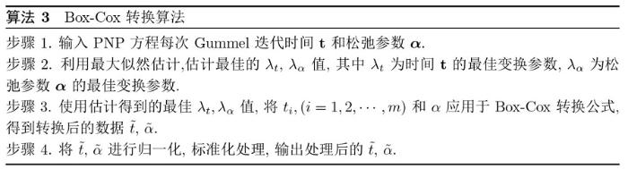
3.2 Box-Cox 转换

对于 PNP 方程的输入样本 $\textbf{t}$ 和 $\boldsymbol{\alpha}$ 可能远离正态分布, 所以本节我们利用 Box-Cox 转换, 将 $\textbf{t}$ 和 $\boldsymbol{\alpha}$ 转化成一个近似的多元高斯分布, 提高 GPR 的准确性. Box-Cox 转换是一种常用的数据变换方法, 用于处理非正态分布的数据或者使数据满足线性回归的假设, Box-Cox 转换通过幂函数将数据进行调整, 将数据的分布转换为更加接近正态分布的形式. 转换公式如下^[11]

$\left\{\begin{aligned} &\tilde{y}=\left(y^{\lambda}-1\right) / \lambda, && \lambda \neq 0, \\ &\tilde{y}=\log (y), && \lambda=0. \end{aligned}\right.$

文献 [11] 指出经过 Box-Cox 变换得到的 $\tilde{y}$ 满足近似分布, $\tilde{y}$ 是转换后的数据, $y$ 是原始数据, $\lambda$ 是转换参数. $\lambda$ 可以取任意实数值, 一般利用最大似然估计法来确定最佳的 $\lambda$ 值.

下面给出具体的 PNP 方程的 Box-Cox 转换算法

3.3 基于 GPR 方法的新 Gummel 迭代算法

下面基于算法 2 和算法 3, 给出基于 GPR 方法选取松弛参数新 Gummel 迭代算法

4 数值实验

为验证新 Gummel 算法的有效性, 本文选取一个三维稳态 PNP 模型, 利用 GPR 方法选取 PNP 方程 Gummel 迭代的较优参数, 并与经典的 Gummel 算法进行比较. 实验环境为个人电脑, CPU 为 2.10GHz, 内存为 32GB, 采用 MATLAB 语言编写计算程序, 所有计算结果均来自同一实验环境.

算例 4.1 考虑方程 (2.1)-(2.3), 其求解区域 $\Omega=[-L / 2,L / 2]^{3}$ , 是一个边长为 Lnm 的正方体区域, 正方体的六个面为边界 $\partial \Omega$ , 真解为^[7]

$\begin{align*} & u_{\mathrm{r}}=\frac{1}{3 \pi^{2} \varepsilon_{s}} \frac{\mathrm{e}_{c}^{2} \beta}{\varepsilon_{0}} c_{\text {bulk }} \cos (\pi x) \cos (\pi y) \cos (\pi z), \\ & p_{\mathrm{r}}=c_{\text {bulk }}\left[1+\frac{1}{2} \cos (\pi x) \cos (\pi y) \cos (\pi z)\right], \\ & n_{\mathrm{r}}=c_{\text {bulk }}\left[1-\frac{1}{2} \cos (\pi x) \cos (\pi y) \cos (\pi z)\right]. \end{align*}$

其中, $c_{\text {bulk }}$ 为模型真解设定浓度, 为 $6.022\times10^{26}{\rm m}^{-3}$ , 即 $10^{-3}$ mol/L.

4.1 无量纲化

本文方程 (2.1)-(2.3) 对应的参数数值及符号如下表所示

表1 参数数值及符号

新窗口打开| 下载CSV

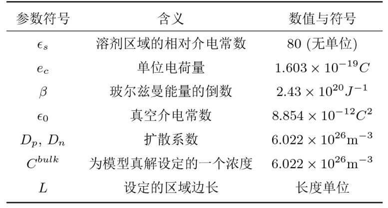
通过无量纲化将方程 (2.1)-(2.3) 转化为 (4.1) 来进行求解.

$\begin{align*}\label{1.4} &-\nabla\cdot\nabla\tilde{u}=(\tilde{p}-\tilde{n}), \\ &-\nabla\cdot(\nabla\tilde{p}+c_{\lambda}\tilde{p}\nabla\tilde{u})=-\nabla\cdot(\nabla\tilde p_{r}+c_{\lambda}\tilde p_{r}\nabla\tilde u_{r}), \\ &-\nabla\cdot(\nabla\tilde{n}+c_{\lambda}\tilde{n}\nabla\tilde{u})=-\nabla\cdot(\nabla\tilde n_{r}+c_{\lambda}\tilde n_{r}\nabla\tilde u_{r}), \end{align*}$

(4.1)

其中当求解区域为 $[-\frac{L}{2},\frac{L}{2}]^{3}, L=0.78$ nm 时, $c_{\lambda}=0.5$ . 边界条件 $\tilde{u}_d, \tilde{p}_d, \tilde{n}_d$ , 真解 $\tilde{u}_r,\tilde{p}_r,\tilde{n}_r$ 变为

$\begin{align*}\label{1.5} &\tilde{u}_{d}=\tilde{u}_{r}=\cos \frac{\pi x}{L} \cos \frac{\pi y}{L} \cos \frac{\pi z}{L}, \\ &\tilde{p}_{d}=\tilde{p}_{r}=3 \pi^{2}\left(1+\frac{1}{2} \cos \frac{\pi x}{L} \cos \frac{\pi y}{L} \cos \frac{\pi z}{L}\right), \\ &\tilde{n}_{d}=\tilde{n}_{r}=3 \pi^{2}\left(1-\frac{1}{2} \cos \frac{\pi x}{L} \cos \frac{\pi y}{L} \cos \frac{\pi z}{L}\right). \end{align*}$

(4.2)

4.2 数值结果

首先利用算法 4 求解方程 (4.1), $t_*$ 选为比训练过程中 Gummel 迭代的迭代时间更小的一个值. 表2 给出了算法 4 的有限元解的 $L^2$ 模误差, 其收敛阶达到二阶, 为最优收敛阶, 与理论结果相符^[12].

表2 算法 4 的解的 $L^2$ 模误差

新窗口打开| 下载CSV

其次比较经典 Gummel 迭代算法 1 与算法 4 的计算效率. 下面图1 中的 (a) 和 (b) 分别给出了算法 4 与算法 1 迭代步数与 CPU 时间, 其中“GPR”(红色-o-线) 表示算法 4 的 Gummel 迭代步数或 CPU 时间, 0.1 到 0.9 为算法 1 中 $\alpha$ 分别取 0.1 到 0.9 的迭代步数或 CPU 时间.

图1

新窗口打开| 下载原图ZIP| 生成PPT

图1 算法 4 与算法 1 迭代次数

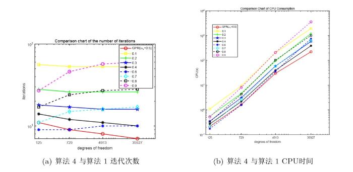
图1 的结果表明, 算法 4 与算法 1 的其他松弛参数取值相比, 在相同的自由度下迭代次数和 CPU 的时间更少, 说明了新 Gummel 算法的有效性. 注意到算法 4 虽然包含算法 2 的训练时间, 但是由于松弛参数 $\alpha$ 使用的是较优的, 所以算法 4 的 CPU 时间更少.

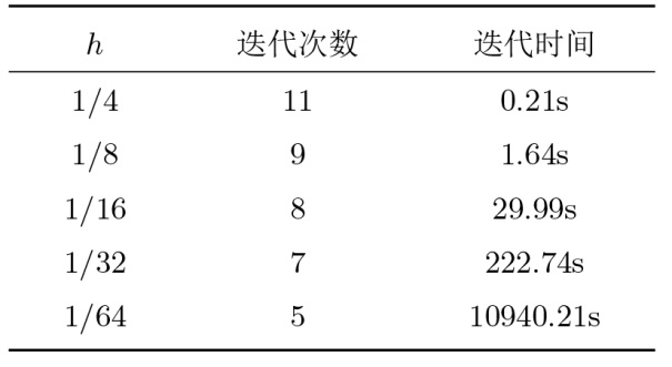
最后, 表3 给出了算法 4 在不同的网格尺度下的迭代次数及 CPU 时间. 结果表明, 随着 $h$ 变小 (问题规模增大), 迭代次数没有增加, 反而呈下降趋势. 这也说明了我们构造的新算法的有效性.

表3 算法 4 的迭代次数与 CPU 时间

新窗口打开| 下载CSV

5 结论

我们研究了利用高斯过程回归方法对 PNP 方程中 Gummel 迭代的松弛参数进行选取, 获得一个较优的松弛参数. 通过对经典的 Gummel 迭代的松弛参数取不同取值进行测试表明, 基于 GPR 方法的新 Gummel 迭代算法, 在 PNP 方程迭代求解过程中, 迭代次数更少, 迭代时间更短.

参考文献

原文顺序

文献年度倒序

文中引用次数倒序

被引期刊影响因子

[1]

B Z

, Holst

M J

, McCammon

J A

et al.

Poisson-Nernst-Planck equations for simulating biomolecular diffusion-reaction processes I: Finite element solutions

Journal of Computational Physics, 2010, 229(19): 6979-6994

PMID:21709855 [本文引用: 1]

In this paper we developed accurate finite element methods for solving 3-D Poisson-Nernst-Planck (PNP) equations with singular permanent charges for electrodiffusion in solvated biomolecular systems. The electrostatic Poisson equation was defined in the biomolecules and in the solvent, while the Nernst-Planck equation was defined only in the solvent. We applied a stable regularization scheme to remove the singular component of the electrostatic potential induced by the permanent charges inside biomolecules, and formulated regular, well-posed PNP equations. An inexact-Newton method was used to solve the coupled nonlinear elliptic equations for the steady problems; while an Adams-Bashforth-Crank-Nicolson method was devised for time integration for the unsteady electrodiffusion. We numerically investigated the conditioning of the stiffness matrices for the finite element approximations of the two formulations of the Nernst-Planck equation, and theoretically proved that the transformed formulation is always associated with an ill-conditioned stiffness matrix. We also studied the electroneutrality of the solution and its relation with the boundary conditions on the molecular surface, and concluded that a large net charge concentration is always present near the molecular surface due to the presence of multiple species of charged particles in the solution. The numerical methods are shown to be accurate and stable by various test problems, and are applicable to real large-scale biophysical electrodiffusion problems.

[2]

Silva

V L S

, Salinas

, Jackson

M D

et al.

Machine learning acceleration for nonlinear solvers applied to multiphase porous media flow

Computer Methods in Applied Mechanics and Engineering, 2021, 384: 113989

DOI:10.1016/j.cma.2021.113989 URL [本文引用: 1]

[3]

Jiang

, Su

X H

, Zhang

A General alternating-direction implicit framework with Gaussian process regression parameter prediction for large sparse linear systems

SIAM Journal on Scientific Computing, 2022, 44(4): A1960-A1988

[本文引用: 1]

[4]

Uyan

O G

, Akbas

, Gungor

V C

Machine Learning Approaches for Underwater Sensor Network Parameter Prediction

Ad Hoc Networks, 2023, 144: 103139

[本文引用: 1]

[5]

Singh

S K

, Das

A K

, Singh

S R

et al.

Prediction of rail-wheel contact parameters for a metro coach using machine learning

Expert Systems with Applications, 2023, 215: 119343

[本文引用: 1]

[6]

S d

, Lu

B Z

INN: Interfaced neural networks as an accessible meshless approach for solving interface PDE problems

Journal of Computational Physics, 2022, 470: 111588

[本文引用: 1]

[7]

Wang

, Li

H L

, Zhang

L B

et al.

A stabilized finite element method for the Poisson-Nernst-Planck equations in three-dimensional ion channel simulations

Applied Mathematics Letters, 2020, 111: 106652

[本文引用: 2]

[8]

Yang

, Tang

, Zhong

L Q

et al.

Superconvergent gradient recovery for nonlinear Poisson-Nernst-Planck equations with applications to the ion channel problem

Advances in Computational Mathematics, 2020, 46(6): 1-35

[9]

Seeger

Gaussian processes for machine learning

International Journal of Neural Systems, 2004, 14(2): 69-106

PMID:15112367 [本文引用: 1]

Gaussian processes (GPs) are natural generalisations of multivariate Gaussian random variables to infinite (countably or continuous) index sets. GPs have been applied in a large number of fields to a diverse range of ends, and very many deep theoretical analyses of various properties are available. This paper gives an introduction to Gaussian processes on a fairly elementary level with special emphasis on characteristics relevant in machine learning. It draws explicit connections to branches such as spline smoothing models and support vector machines in which similar ideas have been investigated. Gaussian process models are routinely used to solve hard machine learning problems. They are attractive because of their flexible non-parametric nature and computational simplicity. Treated within a Bayesian framework, very powerful statistical methods can be implemented which offer valid estimates of uncertainties in our predictions and generic model selection procedures cast as nonlinear optimization problems. Their main drawback of heavy computational scaling has recently been alleviated by the introduction of generic sparse approximations.13,78,31 The mathematical literature on GPs is large and often uses deep concepts which are not required to fully understand most machine learning applications. In this tutorial paper, we aim to present characteristics of GPs relevant to machine learning and to show up precise connections to other "kernel machines" popular in the community. Our focus is on a simple presentation, but references to more detailed sources are provided.

[10]

Williams

C K I

, Rasmussen

C E

Gaussian Processes for Machine Learning. Cambridge: MIT Press, 2006

[本文引用: 1]

[11]

Box

G E P

, Cox

D R

An analysis of transformations

Journal of the Royal Statistical Society: Series B (M ethodological), 1964, 26(2): 211-252

[本文引用: 2]

[12]

Yang

, Lu

B Z

An error analysis for the finite element approximation to the steady-state Poisson-Nernst-Planck equations

Advances in Applied Mathematics and Mechanics, 2013, 5(1): 113-130

[本文引用: 1]

Poisson-Nernst-Planck equations for simulating biomolecular diffusion-reaction processes I: Finite element solutions

2010

... Poisson-Nernst-Planck 方程, 简称为 PNP 方程, 可用来描述生物分子系统的电扩散反应过程, 并且该模型已经被广泛的应用于电化学、半导体、生物膜通道等领域^[1]. 由于 PNP 方程是一个非线性的耦合系统, 常需要利用解耦方法进行求解, 而 Gummel 迭代是一种广泛应用于求解 PNP 方程的解耦方法. 对于实际 PNP 问题, 通常需要利用松弛参数才能保证 Gummel 迭代收敛. 而松弛参数的取值对 Gummel 迭代的收敛效果影响较大, 传统的 Gummel 迭代法都是按照经验来给定松弛参数取值, 然而, 按照经验取值一般不是较优松弛参数, 可能造成 PNP 方程迭代时间很长, 迭代速度很慢. ...

Machine learning acceleration for nonlinear solvers applied to multiphase porous media flow

2021

... 近年来机器学习技术被引入到各种模型的数值计算中, 通过预测出较优参数, 来加速数值解的收敛, 降低数值模拟中的计算成本. 比如 Mukerji 等人^[2] 利用随机森林回归加速多相多孔介质流的求解. Jiang 等人^[3] 引入了高斯过程回归 (GPR) 来预测交替方向隐式方法 (ADI) 中的参数, 以提高求解的效率和准确性. Uyan^[4] 使用机器学习方法来预测水下传感器网络参数, 提高水下传感器网络的性能和可靠性. Sudhir^[5] 使用人工神经网络 (ANN) 和递归神经网络 (RNN) 模型来预测车轮接触参数, 来减少脱轨倾向、车轮磨损和能耗. 我们注意到最近也出现了少量利用机器学习方法求解 PNP 方程的工作, 如文献 [6] 利用接口神经网络方法 (INNs) 求解 PNP 方程, 加速方程收敛和提高数值精度. 但是该文主要侧重于利用机器学习算法求解, 而不是用于预测参数. 据我们所知, 目前还没有利用机器学习来预测 PNP 方程迭代算法参数的相关工作. 本文针对一类 PNP 方程, 利用 GPR 方法对 Gummel 迭代的松弛参数进行预测, 得到较优参数, 提高 Gummel 迭代的收敛效率. 首先, 针对 PNP 方程的 Gummel 迭代设计了 GPR 方法. 其次, 利用 Box-Cox 转换算法, 对 GPR 的训练集进行处理, 使其接近高斯分布, 提高 GPR 方法的准确性. 然后基于 GPR 方法及 Box-Cox 转换算法给出一种新的 Gummel 算法. 数值实验表明: 这一新算法与经典的 Gummel 算法相比, 在收敛阶相同的情况下, 计算效率更高. ...

A General alternating-direction implicit framework with Gaussian process regression parameter prediction for large sparse linear systems

2022

Machine Learning Approaches for Underwater Sensor Network Parameter Prediction

2023

Prediction of rail-wheel contact parameters for a metro coach using machine learning

2023

INN: Interfaced neural networks as an accessible meshless approach for solving interface PDE problems

2022

A stabilized finite element method for the Poisson-Nernst-Planck equations in three-dimensional ion channel simulations

2020

... 本文考虑一种在半导体领域中的 PNP 方程^[7] ...

... 算例 4.1 考虑方程 (2.1)-(2.3), 其求解区域

$\Omega=[-L / 2,L / 2]^{3}$

, 是一个边长为 Lnm 的正方体区域, 正方体的六个面为边界

$\partial \Omega$

, 真解为^[7] ...

Superconvergent gradient recovery for nonlinear Poisson-Nernst-Planck equations with applications to the ion channel problem

2020

Gaussian processes for machine learning

2004

... 本节, 首先参考文献 [9] 的工作设计了针对 PNP 方程的 Gummel 迭代的 GPR 算法. 然后利用 Box-Cox 转换方法, 对 GPR 的训练集进行预处理. 最后我们给出基于 GPR 方法的新 Gummel 迭代算法. ...

2006

... 其中

$\sigma_f$

$l$

是超参数, 可利用极大化边际似然对数函数 L^[10] 来确定 ...

An analysis of transformations

1964

... 对于 PNP 方程的输入样本

$\textbf{t}$

和

$\boldsymbol{\alpha}$

可能远离正态分布, 所以本节我们利用 Box-Cox 转换, 将

$\textbf{t}$

和

$\boldsymbol{\alpha}$

转化成一个近似的多元高斯分布, 提高 GPR 的准确性. Box-Cox 转换是一种常用的数据变换方法, 用于处理非正态分布的数据或者使数据满足线性回归的假设, Box-Cox 转换通过幂函数将数据进行调整, 将数据的分布转换为更加接近正态分布的形式. 转换公式如下^[11] ...

... 文献 [11] 指出经过 Box-Cox 变换得到的

$\tilde{y}$

满足近似分布,

$\tilde{y}$

是转换后的数据,

$y$

是原始数据,

$\lambda$

是转换参数.

$\lambda$

可以取任意实数值, 一般利用最大似然估计法来确定最佳的

$\lambda$

值. ...

An error analysis for the finite element approximation to the steady-state Poisson-Nernst-Planck equations

2013

... 首先利用算法 4 求解方程 (4.1),

$t_*$

选为比训练过程中 Gummel 迭代的迭代时间更小的一个值. 表2 给出了算法 4 的有限元解的

$L^2$

模误差, 其收敛阶达到二阶, 为最优收敛阶, 与理论结果相符^[12]. ...

〈

〉