炭疽是一种由炭疽芽孢杆菌引起的高度致命传染病, 主要感染斑马、跳羚等食草动物^[1], 全球野生动物的死亡主要是由炭疽引起的^[2]. 炭疽通常出现在发展中国家, 如非洲、亚洲的大部分地区, 欧洲和北美南美的部分地区, 即使在发达国家, 偶尔也会爆发炭疽, 炭疽有时也被用于生物恐怖袭击或生物战争^[3], 因此分析炭疽的传播动态极其重要.

世界多个地方都曾出现过动物种群的炭疽大爆发, 引起了许多学者的关注和研究. 1981 年, Furniss 和 Hahn^[4]以克鲁格国家公园爆发的动物炭疽为背景, 建立了差分方程炭疽模型. 2013 年, Friedman 和 Yakubu^[5]在动物种群中建立了一个带有局部扩散的微分方程模型, 研究了尸体摄入、尸体引起的环境污染和迁移率等对动物种群的影响. 2017 年, Saad-Roy 等^[6]通过建立具有 Logistic 增长的炭疽模型来研究动物群体中炭疽的传播, 其研究结果表明, 染病动物的数量与炭疽孢子病毒的数量密切相关. 在近几年的传染病建模中, 媒介在疾病传播过程中的作用越来越受到人们的关注. 从十九世纪开始, 昆虫就被认为是传播炭疽的罪魁祸首, 在二十世纪初,叮咬蝇被认为是疾病传播的重要媒介^[7]. 以往的一些文章中指出在实验条件下至少有 21 种虻科蝇被证实其身体部位携带炭疽杆菌^[8], 表明炭疽能够通过苍蝇进行传播. 2014 年, Blackburn 等^[9]研究了尸食性蝇传播炭疽的方式, 文章中指出当动物感染炭疽死亡后, 由于染病尸体上寄生着寻找食物和产卵的尸食性蝇, 因此, 一方面蛆和苍蝇可能会污染尸体外部及尸体附近的土壤, 另一方面离开尸体的成年苍蝇能够通过呕吐或排便的方式将携带的细菌转移到附近植被, 进而感染食草动物. 此外, 文献[10,11]也对尸食性蝇的传播方式进行了介绍. 2013 年, Baldacchino 等^[12]研究了血食性蝇传播炭疽的方式, 由于血食性蝇叮咬染病动物后嘴部或腿部携带炭疽杆菌, 则之后通过叮咬能够传染易感动物. 2010 年, Blackburn 等^[13]在文章中指出了尸食性蝇和血食性蝇均能够传播炭疽. 2017 年, Mushayabasa 等^[14]在建立动物种群中炭疽的传播模型时加入了血食性蝇, 研究了所建模型的理论结果与媒介对炭疽传播和控制的影响.

在研究媒介对炭疽传播的影响时, 一方面以往的大部分文章虽然介绍了动物种群与尸食性蝇、血食性蝇之间复杂的传播机制, 但是没有建立相应的模型进行分析, 另一方面一些学者只研究了一类苍蝇对动物种群中炭疽传播的影响, 不够全面, 在此基础上, 本文同时考虑了尸食性蝇和血食性蝇两类苍蝇在食草动物中的传播机制, 建立了一个具有两类媒介的动物种群中炭疽传播的数学模型.

本文考虑了十一个仓室, 分别为易感动物 ($S_{a}(t)$), 染病动物 ($I_{a}(t)$), 环境中的孢子病毒 ($P(t)$), 自然死亡的动物尸体 ($S_{c}(t)$), 感染炭疽死亡的动物尸体 ($I_{c}(t)$), 则动物的总数量为$N_{a}(t)=S_{a}(t)+I_{a}(t)$, 尸体的总数量为$N_{c}(t)=S_{c}(t)+I_{c}(t)$. 对于尸食性蝇和血食性蝇两类媒介, 考虑它们的幼虫阶段和成虫阶段, 并将成虫阶段分为两类. 假设尸食性蝇 (血食性蝇) 的幼虫数量为$L_{N}(t)$($L_{H}(t)$), 成虫易感者数量为$S_{N}(t)$($S_{H}(t)$), 成虫染病者数量为$I_{N}(t)$($I_{H}(t)$). 其具体模型为

其中, 易感动物的输入率为$\Lambda_{a}$, 自然死亡率为$d_{a}$,$\beta_{Pa}$是环境中孢子病毒对易感动物的传染率. 由于尸食性蝇从染病尸体上获得孢子病毒后通过污染尸体附近的植被感染食草动物, 血食性蝇通过叮咬染病动物携带孢子病毒进而感染食草动物, 则$\beta_{Ha}$,$\beta_{cN}$和$\beta_{aH}$分别表示染病的血食性蝇对易感动物的传染率、染病尸体对尸食性蝇的传染率和染病动物对血食性蝇的传染率. 染病动物的因病死亡率为$\delta_{a}$,$\eta_{c}$是染病尸体释放孢子病毒的速率, 尸食性蝇感染炭疽后释放到尸体附近植被的孢子病毒的速率为$\eta_{N}$,$\xi$是孢子病毒的衰减率,$\mu_{c}$是尸体的腐烂率. 对于尸食性蝇和血食性蝇两类媒介, 假设感染炭疽不影响产卵率$b_{N}$($b_{H}$) 和死亡率$d_{N}$($d_{H}$), 幼虫期的自然死亡率和成熟率分别为$\mu_{N}$($\mu_{H}$) 和$\Lambda_{N}$($\Lambda_{H}$), 在苍蝇繁殖过程中, 幼虫因拥挤或竞争而死亡的现象很常见,$\alpha_{N}$($\alpha_{H}$) 表示幼虫的密度依赖性发育死亡率. 系统 (2.1) 中所有参数均为正常数. 为了简便, 引入变量$F_{N}(t)=S_{N}(t)+I_{N}(t)$,$F_{H}(t)=S_{H}(t)+I_{H}(t)$, 则系统 (2.1) 的等价系统为

下面证明系统 (2.2) 的有界性.

定理 2.1 对于任意的初值$(S_{a}(0),I_{a}(0),P(0),S_{c}(0),I_{c}(0),L_{N}(0),F_{N}(0),I_{N}(0),L_{H}(0),$$F_{H}(0),I_{H}(0))\in\Omega$, 系统 (2.2) 存在唯一的非负有界解, 其中

此外, 系统 (2.2) 的正向不变集为

证 由文献[15]可知, 对任意的初值$(S_{a}(0),I_{a}(0),P(0),S_{c}(0),I_{c}(0),L_{N}(0),F_{N}(0),I_{N}(0),$$L_{H}(0),F_{H}(0),I_{H}(0))\in\Omega$, 系统 (2.2) 在其最大存在区间$[0,T)$,$T\leq\infty$上存在唯一的非负解. 对于任意的$(S_{a},I_{a},P,S_{c},I_{c},L_{N},F_{N},I_{N},L_{H},F_{H},I_{H})\in\Omega$, 当$I_{N}(t)=F_{N}(t)$,$I_{H}(t)=F_{H}(t)$时, 有$I'_{N}(t)\leq0$,$I'_{H}(t)\leq0$, 由文献[15]可得, 对任意的$t\in[0,T)$,$I_{N}(t)\leq F_{N}(t)$,$I_{H}(t)\leq F_{H}(t)$.

将系统 (2.2) 中的$S_{a}$与$I_{a}$,$S_{c}$与$I_{c}$分别相加可得

则对任意的$t>0$,$N_{a}(t)>0$且$N_{c}(t)>0$, 此时$N_{a}(t)$和$N_{c}(t)$在$t\in[0,T)$上有界.

对于以下系统

由文献[16]可知, 对$\mathbb{R}_{+}^{2}\backslash\{(0,0)\}$中的所有初值, 存在一个全局渐近稳定的平衡点$\left(\frac{b\lambda}{\alpha d},\frac{b}{\alpha}\left(\frac{\lambda}{d}\right)^{2}\right)$. 由于

通过比较原理可知, 在$[0,T)$上$L_{N}(t)$和$F_{N}(t)$有界. 类似地,$L_{H}(t)$和$F_{H}(t)$在$[0,T)$上有界.

注意到$P'(t)=\eta_{c}I_{c}(t)+\eta_{N}I_{N}(t)-\xi P(t)\leq\eta_{c}N_{c}(t)+\eta_{N}F_{N}(t)-\xi P(t)$, 再次使用比较定理可得$P(t)$在$t\in[0,T)$上有界. 因此$T=\infty$,$\Gamma$中的估计不等式可由上面的讨论得到. 定理得证.

从系统 (2.2) 可以看出尸食性蝇满足的方程为

这一系统在文献[17]中已经被研究了. 定义尸食性蝇的媒介再生数为$R_{\nu N}=\frac{b_{N}\Lambda_{N}}{d_{N}(\mu_{N}+\Lambda_{N})}$. 由系统 (2.6) 可知,当$R_{\nu N}\leq1$时, 系统(2.6)存在一个平衡点$(0,0)$, 当$R_{\nu N}>1$时, 系统 (2.6)存在正平衡点$(L_{N}^{\ast},F_{N}^{\ast})$, 其中

血食性蝇满足的方程为

类似地, 定义血食性蝇的媒介再生数为$R_{\nu H}=\frac{b_{H}\Lambda_{H}}{d_{H}(\mu_{H}+\Lambda_{H})}$, 当$R_{\nu H}\leq1$时, 系统 (2.7) 存在一个平衡点$(0,0)$, 当$R_{\nu H}>1$时, 系统 (2.7) 存在一个正平衡点$(L_{H}^{\ast},F_{H}^{\ast})$, 其中

根据文献[17]可知以下结论是成立的.

引理 2.1 (i) 对于系统 (2.6), 若$R_{\nu N}\leq1$, 平衡点$(0,0)$在$\mathbb{R}_{+}^{2}$上是全局渐近稳定的; 若$R_{\nu N}>1$, 正平衡点$(L_{N}^{\ast},F_{N}^{\ast})$在$\mathbb{R}_{+}^{2}\setminus\{(0,0)\}$上是全局渐近稳定的.

(ii) 对于系统 (2.7), 若$R_{\nu H}\leq1$, 平衡点$(0,0)$在$\mathbb{R}_{+}^{2}$上是全局渐近稳定的; 若$R_{\nu H}>1$, 正平衡点$(L_{H}^{\ast},F_{H}^{\ast})$在$\mathbb{R}_{+}^{2}\setminus\{(0,0)\}$上是全局渐近稳定的.

下面计算系统 (2.2) 的平衡点. 显然, 系统 (2.2) 有以下五个平衡点, 分别为

(1)$E_{1}=(S_{a}^{0},0,0,S_{c}^{0},0,0,0,0,0,0,0)$,$S_{a}^{0}=\frac{\Lambda_{a}}{d_{a}}$,$S_{c}^{0}=\frac{\Lambda_{a}}{\mu_{c}}.$

平衡点$E_{1}$是两类苍蝇均不存在时模型的无病平衡点, 且$E_{1}$总存在.

(2)$E_{2}=(S_{a_{2}},I_{a_{2}},P_{2},S_{c_{2}},I_{c_{2}},0,0,0,0,0,0)$, $S_{a_{2}}=\frac{\xi\mu_{c}}{\beta_{Pa}\eta_{c}}$, $I_{a_{2}}=\frac{d_{a}\xi\mu_{c}\left(\frac{\beta_{Pa}\eta_{c}\Lambda_{a}}{\xi\mu_{c}d_{a}}-1\right)}{\beta_{Pa}\eta_{c}(d_{a}+\delta_{a})}$, $P_{2}=\frac{d_{a}}{\beta_{Pa}}\left(\frac{\beta_{Pa}\eta_{c}\Lambda_{a}}{\xi\mu_{c}d_{a}}-1\right)$, $S_{c_{2}}=\frac{d_{a}\xi}{\beta_{Pa}\eta_{c}}$, $I_{c_{2}}=\frac{d_{a}\xi}{\beta_{Pa}\eta_{c}}\left(\frac{\beta_{Pa}\eta_{c}\Lambda_{a}}{\xi\mu_{c}d_{a}}-1\right).$

平衡点$E_{2}$是两类苍蝇均不存在时模型的地方病平衡点, 当且仅当$\frac{\beta_{Pa}\eta_{c}\Lambda_{a}}{\xi\mu_{c}d_{a}}>1$时,$E_{2}$存在.

(3)$E_{3}=(S_{a}^{0},0,0,S_{c}^{0},0,0,0,0,L_{H}^{\ast},F_{H}^{\ast},0)$,$S_{a}^{0}=\frac{\Lambda_{a}}{d_{a}}$,$S_{c}^{0}=\frac{\Lambda_{a}}{\mu_{c}}$,$L_{H}^{\ast}=\frac{\Lambda_{H}+\mu_{H}}{\alpha_{H}}(R_{\nu H}-1)$,$F_{H}^{\ast}=\frac{\Lambda_{H}}{d_{H}}L_{H}^{\ast}$.

平衡点$E_{3}$是只存在血食性蝇时模型的无病平衡点, 当且仅当$R_{\nu H}>1$时,$E_{3}$存在.

(4)$E_{4}=(S_{a}^{0},0,0,S_{c}^{0},0,L_{N}^{\ast},F_{N}^{\ast},0,0,0,0)$,$S_{a}^{0}=\frac{\Lambda_{a}}{d_{a}}$,$S_{c}^{0}=\frac{\Lambda_{a}}{\mu_{c}}$,$L_{N}^{\ast}=\frac{\Lambda_{N}+\mu_{N}}{\alpha_{N}}(R_{\nu N}-1)$,$F_{N}^{\ast}=\frac{\Lambda_{N}}{d_{N}}L_{N}^{\ast}$.

平衡点$E_{4}$是只存在尸食性蝇时模型的无病平衡点, 当且仅当$R_{\nu N}>1$时,$E_{4}$存在.

(5)$E_{5}=(S_{a}^{0},0,0,S_{c}^{0},0,L_{N}^{\ast},F_{N}^{\ast},0,L_{H}^{\ast},F_{H}^{\ast},0),$ $S_{a}^{0}=\frac{\Lambda_{a}}{d_{a}}$, $S_{c}^{0}=\frac{\Lambda_{a}}{\mu_{c}}$, $L_{N}^{\ast}=\frac{\Lambda_{N}+\mu_{N}}{\alpha_{N}}(R_{\nu N}-1)$, $F_{N}^{\ast}=\frac{\Lambda_{N}}{d_{N}}L_{N}^{\ast}$, $L_{H}^{\ast}=\frac{\Lambda_{H}+\mu_{H}}{\alpha_{H}}(R_{\nu H}-1)$, $F_{H}^{\ast}=\frac{\Lambda_{H}}{d_{H}}L_{H}^{\ast}$.

平衡点$E_{5}$是系统 (2.2) 的无病平衡点, 当且仅当$R_{\nu N}>1$,$R_{\nu H}>1$时,$E_{5}$存在.

根据文献[18]和[19], 可以得到各类再生数

其中$R_{A}$为两类蝇均不存在时模型的基本再生数,$R_{N}$为只存在尸食性蝇时模型的基本再生数,$R_{H}$为只存在血食性蝇时模型的基本再生数,$R_{0}$为两类蝇都存在时模型的基本再生数.

系统 (2.2) 的其他平衡点计算如下.

首先计算只存在尸食性蝇时模型的地方病平衡点, 令$L_{H}=F_{H}=I_{H}=0$. 设$E_{6}=(S_{a_{6}},I_{a_{6}},P_{6},S_{c_{6}},I_{c_{6}},L_{N_{6}},F_{N_{6}},I_{N_{6}},0,0,0)$是系统 (2.2) 的平衡点, 由系统 (2.2) 可得:$S_{a_{6}}=\frac{\Lambda_{a}-\mu_{c}I_{c_{6}}}{da}$, $I_{a_{6}}=\frac{\mu_{c}I_{c_{6}}}{d_{a}+\delta_{a}}$, $S_{c_{6}}=\frac{\Lambda_{a}-\mu_{c}I_{c_{6}}}{\mu_{c}}$, $P_{6}=\frac{\eta_{c}I_{c_{6}}+\eta_{N}I_{N_{6}}}{\xi}$, $L_{N_{6}}=L_{N}^{\ast}=\frac{\Lambda_{N}+\mu_{N}}{\alpha_{N}}(R_{\nu N}-1)$, $F_{N_{6}}=F_{N}^{\ast}=\frac{\Lambda_{N}}{d_{N}}L_{N}^{\ast}$, $I_{N_{6}}=\frac{\beta_{cN}F_{N}^{\ast}I_{c_{6}}}{\beta_{cN}I_{c_{6}}+d_{N}S_{c}^{0}}$. 仅考虑$I_{c_{6}}\neq 0$的情况, 则关于$I_{c_{6}}$的方程为

其中$B_{1}=\frac{\beta_{Pa}\beta_{cN}\mu_{c}\eta_{c}}{d_{a}}>0$,$B_{2}=\beta_{cN}\xi\mu_{c}(1-R_{A})+\frac{\beta_{Pa}\mu_{c}}{d_{a}}\left(\frac{\eta_{c}d_{N}\Lambda_{a}}{\mu_{c}}+\eta_{N}\beta_{cN}F_{N}^{\ast}\right)$,$B_{3}=d_{N}\Lambda_{a}\xi\left(1-R_{A}-\frac{\beta_{Pa}\eta_{N}\beta_{cN}F_{N}^{\ast}}{\xi d_{N}d_{a}}\right)$. 易知$B_{3}<0$等价于$R_{N}>1$, 此时方程 (3.1) 存在唯一的正根; 当$B_{3}>0$时可推出$R_{A}<1$, 此时$B_{2}>0$成立, 此时方程 (3.1) 没有正根. 又因为$L_{N}^{\ast}>0$等价于$R_{\nu N}>1$, 则当且仅当$R_{\nu N}>1$,$R_{N}>1$时, 平衡点$E_{6}=(S_{a_{6}},I_{a_{6}},P_{6},S_{c_{6}},I_{c_{6}},L_{N}^{\ast},F_{N}^{\ast},I_{N_{6}}, 0,0,0)$存在.

下面计算只存在血食蝇时模型的地方病平衡点, 令$L_{N}=F_{N}=I_{N}=0$. 系统 (2.2) 的简化系统为

从系统 (3.2) 可以看出当$R_{\nu H}>1$时, 在平衡点处,$L_{H_{7}}=L_{H}^{\ast}=\frac{\Lambda_{H}+\mu_{H}}{\alpha_{H}}(R_{\nu H}-1)$,$F_{H_{7}}= F_{H}^{\ast}=\frac{\Lambda_{H}}{d_{H}}L_{H}^{\ast}$. 记$m_{1}=\beta_{Pa}P+\frac{\beta_{Ha}I_{H}}{S_{a}+I_{a}}$,$m_{2}=\frac{\beta_{aH}I_{a}}{S_{a}+I_{a}}$, 此时 (3.2) 式的平衡点满足下列方程

此时

从而

将方程 (3.5) 代入方程 (3.4) 中有

下面仅考虑$m_{1}\neq0$的情况. 方程 (3.6) 两端同时除以$m_{1}$可得

当$\delta_{a}=0$时, 定义

显然, 当$m_{1}\in[0,+\infty)$时,$g(m_{1})$单调递减, 则当且仅当$g(0)=\frac{\beta_{Pa}\eta_{c}\Lambda_{a}}{\xi\mu_{c}d_{a}}+\frac{\beta_{Ha}F_{H}^{\ast}\beta_{aH}}{d_{H}\Lambda_{a}}>1$,即$R_{H}>1$时, 方程 (3.8) 存在唯一的正根, 即系统 (3.2) 存在唯一的正平衡点. 因此, 当且仅当$R_{\nu H}>1$,$R_{H}>1$时, 平衡点$E_{7}=(S_{a_{7}},I_{a_{7}},P_{7},S_{c_{7}},I_{c_{7}},0,0,0,L_{H}^{\ast},F_{H}^{\ast},I_{H_{7}})$存在.

考虑一般情况, 即$\delta_{a}\geq0$, 整理方程 (3.7) 可以得到

其中

显然$C_{1}>0$,$C_{4}>0\Leftrightarrow R_{H}<1$. 定义$H(z)=z^{3}+\frac{C_{2}}{C_{1}}z^{2}+\frac{C_{3}}{C_{1}}z+\frac{C_{4}}{C_{1}}$,$z_{1}=\frac{-C_{2}+\sqrt{C_{2}^{2}-3C_{1}C_{3}}}{3C_{1}}$, 根据文献[20], 可以得到以下定理.

定理 3.1 假设$\delta_{a}\geq0$,$R_{\nu H}>1$, 则下面的结论成立

(i) 若$R_{H}>1$, 系统 (2.2) 至少存在一个形如$(\tilde{S}_{a},\tilde{I}_{a},\tilde{P},\tilde{S}_{c},\tilde{I}_{c},0,0,0,L_{H}^{\ast},F_{H}^{\ast},\tilde{I}_{H})$的平衡点.

(ii) 若$R_{H}\leq1$且$\triangle=C_{2}^{2}-3C_{1}C_{3}<0$, 系统 (2.2) 不存在形如$(\tilde{S}_{a},\tilde{I}_{a},\tilde{P},\tilde{S}_{c},\tilde{I}_{c},0,0,0,L_{H}^{\ast},$$F_{H}^{\ast},\tilde{I}_{H})$的平衡点.

(iii) 若$R_{H}\leq1$, 则当且仅当$z_{1}>0$且$H(z_{1})\leq0$时, 系统 (2.2) 存在形如$(\tilde{S}_{a},\tilde{I}_{a},\tilde{P},\tilde{S}_{c},\tilde{I}_{c},$$0,0,0,L_{H}^{\ast},F_{H}^{\ast},\tilde{I}_{H})$的平衡点.

最后, 计算系统 (2.2) 的正平衡点. 设$n_{1}=\beta_{Pa}P+\frac{\beta_{Ha}I_{H}}{S_{a}+I_{a}}$,$n_{2}=\frac{\beta_{cN}I_{c}}{S_{c}+I_{c}}$,$n_{3}=\frac{\beta_{aH}I_{a}}{S_{a}+I_{a}}$, 讨论过程与上述方法相同, 可知当$\delta_{a}=0$时, 若$R_{\nu N}>1$,$R_{\nu H}>1$,$R_{0}>1$均成立, 则系统 (2.2) 存在唯一的正平衡点$E_{8}=(S_{a_{8}},I_{a_{8}},P_{8},S_{c_{8}},I_{c_{8}},L_{N}^{\ast},F_{N}^{\ast},I_{N_{8}},L_{H}^{\ast},F_{H}^{\ast},I_{H_{8}})$. 对于一般情况, 即$\delta_{a}\geq0$, 定义

其中

依据文献[21]定义$p=\frac{D_{2}}{D_{1}}$, $q=\frac{D_{3}}{D_{1}}$, $u=\frac{D_{4}}{D_{1}}$, $v=\frac{D_{5}}{D_{1}}$, $p_{1}=\frac{q}{2}-\frac{3}{16}p^{2}$, $q_{1}=\frac{p^{3}}{32}-\frac{pq}{8}+u$, $D=\left(\frac{q_{1}}{2}\right)^{2}+\left(\frac{p_{1}}{3}\right)^{3}$, $\sigma=\frac{-1+\sqrt{3}i}{2}$,$y_{1}=\sqrt [3]{-\frac{q_{1}}{2}+\sqrt{D}}+\sqrt[3]{-\frac{q_{1}}{2}-\sqrt{D}}$, $y_{2}=\sqrt[3]{-\frac{q_{1}}{2}+\sqrt{D}}\sigma+\sqrt[3]{-\frac{q_{1}}{2}-\sqrt{D}}\sigma^{2}$, $y_{3}=\sqrt[3]{-\frac{q_{1}}{2}+\sqrt{D}}\sigma^{2}+\sqrt[3]{-\frac{q_{1}}{2}-\sqrt{D}}\sigma$, $w_{i}=y_{i}-\frac{3p}{4},i=1,2,3$. 易知$v>0$等价于$R_{0}<1$. 由文献[21]可以得到以下定理.

定理 3.2 假设$R_{\nu N}>1$,$R_{\nu H}>1$, 则下面结论成立

(i) 如果$R_{0}>1$, 系统 (2.2) 至少存在一个正平衡点.

(ii) 如果$R_{0}\leq1$且$D\geq0$, 当且仅当$w_{1}>0$,$Y(w_{1})<0$时系统 (2.2) 存在正平衡点.

(iii) 如果$R_{0}\leq1$且$D<0$, 系统 (2.2) 存在正平衡点当且仅当至少存在一个$w^{\ast}\in\{w_{1},w_{2},w_{3}\}$, 使得$w^{\ast}>0$且$Y(w^{\ast})\leq0$.

下面分析系统 (2.2) 平衡点的局部渐近稳定性. 由于平衡点$E_{6}$,$E_{7}$和$E_{8}$的稳定性不易分析, 因此只考虑$\delta_{a}=0$的情况.

定理 4.1 平衡点$E_{1}=(S_{a}^{0},0,0,S_{c}^{0},0,0,0,0,0,0,0)$, $E_{2}=(S_{a_{2}},I_{a_{2}},P_{2},S_{c_{2}},I_{c_{2}},0,0,0, 0,$ $0,0)$, $E_{4}=(S_{a}^{0},0,0,S_{c}^{0},0,L_{N}^{\ast},F_{N}^{\ast},0,0,0,0)$和$E_{6}=(S_{a_{6}},I_{a_{6}},P_{6},S_{c_{6}},I_{c_{6}},L_{N}^{\ast},F_{N}^{\ast},I_{N_{6}},0, 0,0)$局部渐近稳定的条件如下

(i) 当$R_{A}<1$,$R_{\nu N}<1$且$R_{\nu H}<1$时, 平衡点$E_{1}$局部渐近稳定; 若$R_{A}>1$或$R_{\nu N}>1$或$R_{\nu H}>1$, 平衡点$E_{1}$不稳定.

(ii) 当$R_{A}>1$时, 平衡点$E_{2}$存在. 若$R_{\nu N}<1$,$R_{\nu H}<1$, 平衡点$E_{2}$局部渐近稳定; 若$R_{\nu N}>1$或$R_{\nu H}>1$, 平衡点$E_{2}$不稳定.

(iii) 当$R_{\nu N}>1$时, 平衡点$E_{4}$存在. 若$R_{\nu H}<1$,$R_{N}<1$, 平衡点$E_{4}$局部渐近稳定; 若$R_{\nu H}>1$或$R_{N}>1$, 平衡点$E_{4}$不稳定.

(iv) 当$R_{N}>1$且$R_{\nu N}>1$时, 平衡点$E_{6}$存在. 当$\delta_{a}=0$时, 若$R_{\nu H}<1$, 平衡点$E_{6}$局部渐近稳定; 若$R_{\nu H}>1$, 平衡点$E_{6}$不稳定.

证 对于平衡点$E_{1}$, 其雅可比矩阵的形式为

其中

由分块矩阵的性质可知,$J(E_{1})$的特征值由$\tilde{J}_{11}$和$\tilde{J}_{22}$的特征值组成.$\tilde{J}_{11}$的特征方程为

其中$I_{5\times5}$是五阶单位矩阵, 且

$-M_{1}$的顺序主子式为$\tilde{\triangle}_{1}=d_{a}+\delta_{a}$,$\tilde{\triangle}_{2}=\xi(d_{a}+\delta_{a})$,$\tilde{\triangle}_{3}=(d_{a}+\delta_{a})\xi\mu_{c}(1-R_{A})$,$\tilde{\triangle}_{4}=\tilde{\triangle}_{3}(\mu_{N}+\Lambda_{N})$,$\tilde{\triangle}_{5}=\tilde{\triangle}_{3}d_{N}(\mu_{N}+\Lambda_{N})(1-R_{\nu N})$, 当且仅当$R_{A}<1$,$R_{\nu N}<1$成立时,$-M_{1}$的顺序主子式均大于零. 又因为$-M_{1}$的主对角线元素均大于零, 非主对角线元素非正, 则$-M_{1}$是 M-矩阵. 由文献[22]可知, 若$R_{A}<1$,$R_{\nu N}<1$成立,$-M_{1}$的所有特征根均具有正实部, 即$M_{1}$的所有特征根均具有负实部. 由于方程 (4.1) 的另外两个特征根为$-\mu_{c}$和$-d_{a}$, 则当$R_{A}<1$,$R_{\nu N}<1$时,$\tilde{J}_{11}$的所有特征根均具有负实部.

$\tilde{J}_{22}$的特征方程为

显然, 当且仅当$d_{H}(\mu_{H}+\Lambda_{H})-\Lambda_{H}b_{H}>0$即$R_{\nu H}<1$时,$\tilde{J}_{22}$的所有特征根均具有负实部.

综上所述, 当且仅当$R_{A}<1$,$R_{\nu N}<1$且$R_{\nu H}<1$时, 平衡点$E_{1}$是局部渐近稳定的.

对于平衡点$E_{2}$和$E_{4}$, 其局部渐近稳定性的证明方法与$E_{1}$相同, 证明过程不再重复. 由于平衡点$E_{6}$的稳定性不易证明, 因此在证明稳定性时只考虑$\delta_{a}=0$的情况. 利用同样的思想, 可以得到: 当平衡点$E_{6}$存在时, 若$R_{\nu H}<1$, 则平衡点$E_{6}$是局部渐近稳定的. 证毕.

定理 4.2 平衡点$E_{3}=(S_{a}^{0},0,0,S_{c}^{0},0,0,0,0,L_{H}^{\ast},F_{H}^{\ast},0)$, $E_{5}=(S_{a}^{0},0,0,S_{c}^{0},0,L_{N}^{\ast},F_{N}^{\ast},0,$ $L_{H}^{\ast},F_{H}^{\ast},0)$, $E_{7}=(S_{a_{7}},I_{a_{7}},P_{7},S_{c_{7}},I_{c_{7}},0,0,0,L_{H}^{\ast},F_{H}^{\ast},I_{H_{7}})$ 和 $E_{8}=(S_{a_{8}},I_{a_{8}},P_{8},S_{c_{8}},I_{c_{8}},L_{N}^{\ast},$ $F_{N}^{\ast},I_{N_{8}},L_{H}^{\ast},F_{H}^{\ast},I_{H_{8}})$局部渐近稳定的条件如下

(i) 当$R_{\nu H}>1$时, 平衡点$E_{3}$存在. 若$R_{\nu N}<1$,$R_{A}<1$, 平衡点$E_{3}$局部渐近稳定; 若$R_{\nu N}>1$或$R_{A}>1$, 平衡点$E_{3}$不稳定.

(ii) 当$R_{\nu N}>1$且$R_{\nu H}>1$时, 系统 (2.2) 的无病平衡点$E_{5}$存在. 若$R_{0}<1$, 平衡点$E_{5}$局部渐近稳定; 若$R_{0}>1$, 平衡点$E_{5}$不稳定.

(iii) 假设$\delta_{a}=0$, 当$R_{\nu H}>1$且$R_{H}>1$时, 平衡点$E_{7}$存在. 若$R_{\nu N}<1$, 平衡点$E_{7}$局部渐近稳定; 若$R_{\nu N}>1$, 平衡点$E_{7}$不稳定.

(iv) 假设$\delta_{a}=0$, 当$R_{\nu N}>1$,$R_{\nu H}>1$且$R_{0}>1$时, 系统 (2.2) 的地方病平衡点$E_{8}$存在, 此时平衡点$E_{8}$局部渐近稳定.

证 对于平衡点$E_{3}$, 它的特征方程为

其中$I_{9\times9}$是九阶单位矩阵, 且

其中,$a_{99}=\mu_{H}+\Lambda_{H}+2\alpha_{H}L_{H}^{\ast}$. $-M_{2}$的顺序主子式为$\bar{\triangle}_{1}=d_{a}+\delta_{a}$, $\bar{\triangle}_{2}=\xi(d_{a}+\delta_{a})$, $\bar{\triangle}_{3}=\xi\mu_{c}(d_{a}+\delta_{a})(1-R_{A})$, $\bar{\triangle}_{4}=\bar{\triangle}_{3}(\mu_{N}+\Lambda_{N})$, $\bar{\triangle}_{5}=\bar{\triangle}_{3}d_{N}(\mu_{N}+\Lambda_{N})(1-R_{\nu N})$, $\bar{\triangle}_{6}=\bar{\triangle}_{5}d_{N}$, $\bar{\triangle}_{7}=\bar{\triangle}_{6}(\mu_{H}+\Lambda_{H}+2\alpha_{H}L_{H}^{\ast})$, $\bar{\triangle}_{8}=\bar{\triangle}_{6}d_{H}(\mu_{H}+\Lambda_{H})(R_{\nu H}-1)$, $\bar{\triangle}_{9}=\bar{\triangle}_{8}d_{H}-\frac{\beta_{Ha}\beta_{aH}F_{H}^{\ast}\xi\mu_{c}d_{N}}{S_{a}^{0}}d_{N}(\mu_{N}+\Lambda_{N})(R_{\nu N}-1)d_{H}(\mu_{H}+\Lambda_{H})(R_{\nu H}-1)$, 当且仅当$R_{A}<1$,$R_{\nu N}<1$且$R_{\nu H}>1$成立时,$-M_{2}$的顺序主子式均大于零. 又因为$-M_{2}$的主对角线元素均大于零, 非主对角线元素非正, 则$-M_{2}$是 M-矩阵. 由文献[22]可知, 若$R_{A}<1$,$R_{\nu N}<1$且$R_{\nu H}>1$成立, 则$-M_{2}$的所有特征根均具有正实部, 即$M_{2}$的所有特征根均具有负实部. 由于方程 (4.3) 的另外两个特征根为$-\mu_{c}$和$-d_{a}$, 则当平衡点$E_{3}$存在时, 若$R_{A}<1$且$R_{\nu N}<1$, 平衡点$E_{3}$局部渐近稳定.

类似地, 可以证明该定理中的结论 (ii), (iii) 和 (iv). 证毕.

定理 4.3 平衡点$E_{1}=(S_{a}^{0},0,0,S_{c}^{0},0,0,0,0,0,0,0)$和$E_{2}=(S_{a_{2}},I_{a_{2}},P_{2},S_{c_{2}},I_{c_{2}},0,0,0,$$0,0,0)$全局渐近稳定的条件如下

(i) 若$R_{\nu N}<1$,$R_{\nu H}<1$且$R_{A}<1$, 则平衡点$E_{1}$在$\Omega$内部全局渐近稳定.

(ii) 若$R_{\nu N}<1$,$R_{\nu H}<1$且$R_{A}>1$, 则平衡点$E_{2}$在$\Omega$内部全局渐近稳定.

证 (i) 由引理 2.1 可知, 若$R_{\nu N}<1$,$R_{\nu H}<1$, 则当$t\rightarrow\infty$时有$(L_{N}(t),F_{N}(t))\rightarrow(0,0)$,$(L_{H}(t),F_{H}(t))\rightarrow(0,0)$, 此时$I_{N}(t)\rightarrow0$,$I_{H}(t)\rightarrow0$, 系统 (2.2) 的极限系统为

由定理 4.1 可知, 当$R_{A}<1$,$R_{\nu N}<1$且$R_{\nu H}<1$时, 平衡点$E_{1}$局部渐近稳定. 由于$R_{A}=\frac{\beta_{Pa}\eta_{c}\Lambda_{a}}{d_{a}\mu_{c}\xi}<1$, 则存在充分小的$\varepsilon>0$, 使得$\frac{\beta_{Pa}\eta_{c}(\frac{\Lambda_{a}}{d_{a}}+\varepsilon)}{\mu_{c}\xi}<1$. 由式 (2.3) 可知$\mathop{\limsup}\limits_{t\rightarrow\infty}N_{a}(t)\leq \frac{\Lambda_{a}}{d_{a}}$, 则存在充分大的$t>0$, 使得$N_{a}(t)\leq\frac{\Lambda_{a}}{d_{a}}+\varepsilon$. 构造 Lyapunov 函数

沿系统 (4.4) 的轨线求$V_{1}$的全导数可得

当$R_{A}<1$时$V'_{1}\leq0$, 且$V'_{1}=0$当且仅当$P=0$成立, 此时有$I_{c}=0$, 从而当$t\rightarrow\infty$时, 有$S_{a}(t)\rightarrow S_{a}^{0}$,$I_{a}(t)\rightarrow 0$,$S_{c}(t)\rightarrow S_{c}^{0}$. 因此,$V'_{1}=0$的唯一紧不变子集为$\{\tilde{E}_{1}=(S_{a}^{0},0,0,S_{c}^{0},0)\}$. 由 LaSalle 不变集原理^[23]可知$\tilde{E}_{1}=(S_{a}^{0},0,0,S_{c}^{0},0)$在$\mathbb{R}_{+}^{5}$上是全局渐近稳定的. 利用内链传递集理论^[24]可知$E_{1}=(S_{a}^{0},0,0,S_{c}^{0},0,0,0,0,0,0,0)$全局渐近稳定.

(ii) 由 (i) 可以看出, 当$R_{\nu N}<1$,$R_{\nu H}<1$时, 系统 (4.4) 为系统 (2.2) 的极限系统. 为了简化系统, 引入新的变量, 令

系统 (4.4) 变为如下形式

定义 Lyapunov 函数$V_{2}$: Int$(\mathbb{R}_{+}^{5})\mapsto \mathbb{R}$

沿系统 (4.5) 的轨线求$V_{2}$的全导数可得

当且仅当$x_{1}=x_{2}=x_{3}=x_{5}=1$时$V'_{2}=0$. 结合系统 (4.5) 得当$t\rightarrow\infty$时$x_{4}\rightarrow1$. 由 LaSalle 不变集原理^[23]可知,$S_{a}(t)\rightarrow S_{a_{2}}$,$I_{a}(t)\rightarrow I_{a_{2}}$,$P(t)\rightarrow P_{2}$,$S_{c}(t)\rightarrow S_{c_{2}}$,$I_{c}(t)\rightarrow I_{c_{2}}$. 利用内链传递集理论^[24]可知$E_{2}=(S_{a_{2}},I_{a_{2}},P_{2},S_{c_{2}},I_{c_{2}},0,0,0,0,0,0)$全局渐近稳定. 证毕.

定理 4.4 平衡点$E_{3}=(S_{a}^{0},0,0,S_{c}^{0},0,0,0,0,L_{H}^{\ast},F_{H}^{\ast},0)$, $E_{4}=(S_{a}^{0},0,0,S_{c}^{0},0,L_{N}^{\ast},F_{N}^{\ast},0,0,$ $0,0)$ 和$E_{5}=(S_{a}^{0},0,0,S_{c}^{0},0,L_{N}^{\ast},F_{N}^{\ast},0,L_{H}^{\ast},F_{H}^{\ast},0)$全局渐近稳定的条件如下

(i) 若$R_{\nu H}>1$,$R_{\nu N}<1$且

则平衡点$E_{3}$在$\Omega$内部是全局渐近稳定的.

(ii) 若$R_{\nu N}>1$,$R_{\nu H}<1$,$R_{N}<1$且

则平衡点$E_{4}$在$\Omega$内部是全局渐近稳定的.

(iii) 若$R_{\nu N}>1$,$R_{\nu H}>1$,$R_{0}<1$且

则平衡点$E_{5}$在$\Omega$内部是全局渐近稳定的.

证 由定理 4.2 可知, 若$R_{\nu H}>1$,$R_{\nu N}<1$且$R_{A}<1$成立, 平衡$E_{3}$是局部渐近稳定的. 由引理 2.1 可得, 若$R_{\nu N}<1$,$R_{\nu H}>1$, 则当$t\rightarrow\infty$时有$(L_{N}(t),F_{N}(t))\rightarrow(0,0)$,$(L_{H}(t),F_{H}(t))\rightarrow(L_{H}^{\ast},F_{H}^{\ast})$, 从而当$t\rightarrow\infty$时可得$I_{N}(t)\rightarrow0$, 此时, 系统 (2.2) 的极限系统为

由系统 (4.6) 的前两个方程可得:$\Lambda_{a}-(d_{a}+\delta_{a})N_{a}(t)\leq N'_{a}(t)\leq\Lambda_{a}-d_{a}N_{a}(t)$, 因此

其中$\phi_{1}=\frac{\Lambda_{a}}{d_{a}+\delta_{a}}$,$S_{a}^{0}=\frac{\Lambda_{a}}{d_{a}}$. 当$t$充分大时有

考虑系统 (4.7) 的辅助系统

定义

显然,$-J$的顺序主子式为$\check{\triangle}_{1}=d_{a}+\delta_{a}$,$\check{\triangle}_{2}=\xi(d_{a}+\delta_{a})$, $\check{\triangle}_{3}=\xi\mu_{c}(d_{a}+\delta_{a})(1-R_{A})$, $\check{\triangle}_{4}=\xi\mu_{c}(d_{a}+\delta_{a})d_{H}\left(1-R_{A}-\left(\frac{d_{a}+\delta_{a}}{d_{a}}\right)^{2}\frac{\beta_{Ha}\beta_{aH}F_{H}^{\ast}}{d_{H}S_{a}^{0}(d_{a}+\delta_{a})}\right)$. 当$R_{A}+\left(\frac{d_{a}+\delta_{a}}{d_{a}}\right)^{2}\frac{\beta_{Ha}\beta_{aH}F_{H}^{\ast}}{d_{H}S_{a}^{0}(d_{a}+\delta_{a})}<1$时, $\check{\triangle}_{3}>0$,$\check{\triangle}_{4}>0$. 定义

易知$R_{A}+\left(\frac{d_{a}+\delta_{a}}{d_{a}}\right)^{2}\frac{\beta_{Ha}\beta_{aH}F_{H}^{\ast}}{d_{H}S_{a}^{0}(d_{a}+\delta_{a})}<1$等价于$R_{H}<\tilde{R}_{c}$, 则当$R_{H}<\tilde{R}_{c}$,$-J$的顺序主子式均大于零. 又因为$-J$的主对角线元素大于零, 非主对角线元素非正, 则$-J$为 M-矩阵, 此时系统 (\ref{4.8}) 的平衡点$(0,0,0,0)$局部渐近稳定, 由于系统 (4.8) 是一个线性系统, 则平衡点$(0,0,0,0)$在$\mathbb{R}_{+}^{4}$上全局渐近稳定. 由比较原理可知, 当$t\rightarrow\infty$时有$(I_{a},P,I_{c},I_{H})\rightarrow(0,0,0,0)$, 从而当$t\rightarrow\infty$时, 有$S_{a}(t)\rightarrow S_{a}^{0}$,$S_{c}(t)\rightarrow S_{c}^{0}$. 因此, 当$R_{\nu H}>1$,$R_{\nu N}<1$且$R_{H}<\tilde{R}_{c}$时, 平衡点$E_{3}$全局渐近稳定.

采用类似的方法可以证明结论 (ii) 和 (iii). 证毕.

推论 4.1 假设$\delta_{a}=0$, 此时$\tilde{R}_{c}=1$, 从而若$R_{\nu H}>1$,$R_{\nu N}<1$且$R_{H}<1$成立, 平衡点$E_{3}$在$\Omega$内部是全局渐近稳定的.

推论 4.2 假设$\delta_{a}=0$, 此时$\hat{R}_{c}=1$, 从而若$R_{N}<1$,$R_{\nu N}>1$且$R_{\nu H}<1$成立, 平衡点$E_{4}$在$\Omega$内部是全局渐近稳定的.

推论 4.3 假设$\delta_{a}=0$, 此时$R_{A}+\left(\frac{d_{a}+\delta_{a}}{d_{a}}\right)\frac{\beta_{Pa}\beta_{cN}\eta_{N}F_{N}^{\ast}}{\xi d_{a}d_{N}}+\left(\frac{d_{a}+\delta_{a}}{d_{a}}\right)^{2}\frac{\beta_{aH}\beta_{Ha}d_{a}F_{H}^{\ast}}{\Lambda_{a}d_{H}(d_{a}+\delta_{a})}<1$等价于$R_{0}<1$, 从而若$R_{\nu N}>1$,$R_{\nu H}>1$且$R_{0}<1$, 平衡点$E_{5}$在$\Omega$内部是全局渐近稳定的.

由于系统 (2.2) 的维数比较高, 很难确定平衡点$E_{6}$,$E_{7}$和$E_{8}$的全局稳定性, 因此, 仅在$\delta_{a}=0$的情况下对其全局稳定性进行研究.

定理 4.5 假设$\delta_{a}=0$, 则平衡点$E_{6}=(S_{a_{6}},I_{a_{6}},P_{6},S_{c_{6}},I_{c_{6}},L_{N}^{\ast},F_{N}^{\ast},I_{N_{6}},0,0,0)$, $E_{7}=(S_{a_{7}},I_{a_{7}},P_{7},S_{c_{7}},I_{c_{7}},0,0,0,L_{H}^{\ast},F_{H}^{\ast},I_{H_{7}})$ 和$E_{8}=(S_{a_{8}},I_{a_{8}},P_{8},S_{c_{8}},I_{c_{8}},L_{N}^{\ast},F_{N}^{\ast},I_{N_{8}},L_{H}^{\ast},F_{H}^{\ast},$ $I_{H_{8}})$全局渐近稳定的条件如下

(i) 若$R_{\nu N}>1$,$R_{N}>1$且$R_{\nu H}<1$, 则平衡点$E_{6}$在$\Omega$内部是全局渐近稳定的.

(ii) 若$R_{\nu H}>1$,$R_{H}>1$且$R_{\nu N}<1$, 则平衡点$E_{7}$在$\Omega$内部是全局渐近稳定的.

(iii) 若$R_{\nu N}>1$,$R_{\nu H}>1$且$R_{0}>1$, 则平衡点$E_{8}$在$\Omega$内部是全局渐近稳定的.

证 由定理 4.1 可知当$\delta_{a}=0$时, 若$R_{N}>1$,$R_{\nu N}>1$且$R_{\nu H}<1$, 平衡点$E_{6}$是局部渐近稳定的. 由引理 2.1 可知, 若$R_{\nu N}>1$,$R_{\nu H}<1$, 则当$t\rightarrow\infty$时有$(L_{N}(t),F_{N}(t))\rightarrow(L_{N}^{\ast},F_{N}^{\ast})$,$(L_{H}(t),F_{H}(t))\rightarrow(0,0)$, 从而当$t\rightarrow\infty$时可得$I_{H}(t)\rightarrow 0$. 由系统 (2.2) 得

显然, 当$t\rightarrow\infty$时,$(N_{a}(t),N_{c}(t))\rightarrow(S_{a}^{0},S_{c}^{0})$, 系统 (4.9) 的唯一正平衡点$(S_{a}^{0},S_{c}^{0})$是全局渐近稳定的, 此时系统 (2.2) 的极限系统为

设$K:=[S_{a}^{0}]\times[\frac{\eta_{c}S_{c}^{0}+\eta_{N}F_{N}^{\ast}}{\xi}]\times[S_{c}^{0}]\times[F_{N}^{\ast}]$, 则$\omega((I_{a}(0),P(0),I_{c}(0),I_{H}(0)))\subset K$, 其中$\omega((I_{a}(0),P(0),I_{c}(0),I_{H}(0)))$是$(I_{a}(0),P(0),I_{c}(0),I_{H}(0))\in \mathbb{R}_{+}^{4}$对于系统 (4.10) 的解半流的$\omega$极限集. 设

则$f:\mathbb{R}_{+}^{4}\rightarrow \mathbb{R}^{4}$是一个连续可微映射, 此外$f$具有以下性质

(1)$f$在$K$上是合作的, 且对任一$v\in K$,$Df(v)=\left(\frac{\partial f_{i}}{\partial v_{j}}\right)_{1\leq i,j\leq4}$是不可约的;

(2) 对于所有的$v\in K$,$f(0)=0$且当$v_{i}=0$时,$f_{i}(v)\geq0$,$i=1,2,3,4$;

(3) 对任意的$\rho\in(0,1)$,$(v_{1},v_{2},v_{3},v_{4})\in$Int$K$, 有

类似可得$f_{2}(\rho v_{1},\rho v_{2},\rho v_{3},\rho v_{4})=\rho f_{2}(v_{1},v_{2},v_{3},v_{4})$, $f_{3}(\rho v_{1},\rho v_{2},\rho v_{3},\rho v_{4})=\rho f_{3}(v_{1},v_{2},v_{3},v_{4})$, $f_{4}(\rho v_{1},\rho v_{2},\rho v_{3},\rho v_{4})>\rho f_{4}(v_{1},v_{2},v_{3},v_{4})$, 则$f$在$K$上是严格次线性的.

由于

则

定义$Df(0)$的谱界为

易知当$R_{A}+\frac{\beta_{Pa}\beta_{cN}F_{N}^{\ast}\eta_{N}}{\xi d_{a}d_{N}}>1$即$R_{N}>1$时, det$(Df(0))<0$,$Df(0)$至少存在一个正的特征值, 从而$s(Df(0))>0$. 由文献[16]可知, 若$R_{N}>1$, 系统 (4.10) 的正平衡点$(I_{a_{6}},P_{6},I_{c_{6}},I_{H_{6}})$在$\mathbb{R}_{+}^{4}\setminus\{(0,0,0,0)\}$中是全局渐近稳定的. 从而, 当$t\rightarrow\infty$时,

因此, 当$\delta_{a}=0$时, 若$R_{N}>1$,$R_{\nu N}>1$且$R_{\nu H}<1$, 平衡点$E_{6}$全局渐近稳定.

类似可以证明平衡点$E_{7}$和平衡点$E_{8}$的全局稳定性. 证毕.

定理 4.5 中讨论了$\delta_{a}=0$时正平衡点的全局稳定性, 对于$\delta_{a}\geq0$的一般情况, 正平衡点的全局稳定性不易得到, 下面的定理给出了疾病的持久性.

若$R_{\nu N}>1$,$R_{\nu H}>1$,$R_{0}>1$, 则存在一个$\epsilon>0$, 使得对于系统 (2.2) 中$I_{a}(0)>0$,$P(0)>0$,$I_{c}(0)>0$,$I_{N}(0)>0$,$I_{H}(0)>0$的所有解满足

证 定理 4.6 的证明过程与文献[25,26]类似, 这里不再赘述.

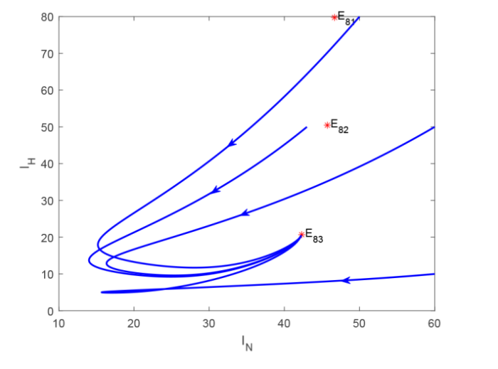
上面在证明平衡点${{E}_{7}}$和${{E}_{8}}$存在性时发现, 当染病食草动物的因病死亡率${{\delta }_{a}}\ge 0$时不止存在一个此类型的平衡点, 并且在证明其稳定性时, 仅仅分析了${{\delta }_{a}}=0$时的特殊情况, 不够全面, 下面以${{E}_{8}}$为例, 给出系统 (2.2) 相应的参数值, 通过数值模拟分析其稳定性情况. 令$\Lambda_{a}=1$, $\beta_{Pa}=0.001$, $\beta_{Ha}=0.02$, $d_{a}=\frac{1}{800}$, $\delta_{a}=\frac{1}{10}$, $\eta_{c}=0.002$, $\eta_{N}=0.01$, $\xi=\frac{1}{10}$, $\mu_{c}=0.05$, $b_{N}=3$, $\mu_{N}=0.1$, $\Lambda_{N}=\frac{1}{16}$, $\alpha_{N}=0.05$, $b_{H}=3$, $\mu_{H}=0.1$, $\Lambda_{H}=\frac{1}{16}$, $\alpha_{H}=0.05$, $\beta_{cN}=0.01$, $\beta_{aH}=0.05$, $d_{N}=\frac{1}{30}$, $d_{H}=\frac{1}{30}$. 此时$R_{vN}=34.6154>1$, $R_{vH}=34.6154>1$, $R_{0}=2.4>1$, 系统 (2.2) 存在三个正平衡点, 分别为:$E_{81}=(13.132,9.7144,5.0607,0.3283,19.6717,109.25,$$204.8438,46.6725,109.25,204.8438,79.7719)$, $E_{82}=(33.9559,9.4573,4.9543,$$0.8489,19.1511,$$109.25,$$204.8438,45.713,109.25,204.8438,50.4506)$, $E_{83}=(105.8201,$$8.5701,$$4.5781,$$2.6455,$$17.3545,$$109.25,204.8438,42.3103,109.25,204.8438,20.6947)$. 由图 1 可以看出, 正平衡点$E_{83}$是渐近稳定的, 正平衡点$E_{81}$和$E_{82}$是不稳定的.

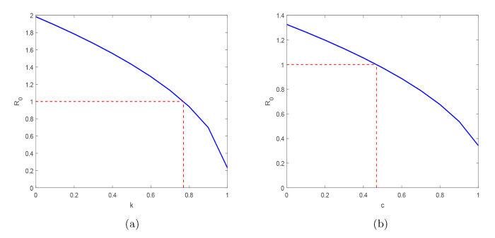
为了降低炭疽导致的食草动物的发病率和死亡率, 探讨不同因素对炭疽传播的影响是非常重要的. 为此, 讨论一些参数与$R_{0}$的关系, 以及控制炭疽传播的可能措施.

由于尸食性蝇和血食性蝇均能传播炭疽, 因此叮咬率对炭疽的传播起着非常重要的作用. 对于尸食性蝇, 为了模拟防止染病尸体被尸食性蝇叮咬导致炭疽传播的效果, 在模型中使用$(1-k)\beta_{cN}$代替$\beta_{cN}$, 其中$\Lambda_{a}=0.1$,$\beta_{Pa}=0.01$,$\beta_{Ha}=0.2$,$\eta_{N}=0.001$,$\mu_{c}=0.1$,$b_{N}=0.3$,$b_{H}=0.3$,$\beta_{cN}=0.1$,$\beta_{aH}=0.015$,其余参数值与图 1 中的参数值相同. 图 2(a) 显示了干预措施$k$与基本再生数$R_{0}$的关系, 其中$R_{0}$是关于$k$的递减函数. 因此, 可以通过清除动物尸体, 减少尸食性蝇的食物来源等方法对炭疽传播进行控制.

对于血食性蝇, 为了模拟易感动物被血食性蝇叮咬导致炭疽传播的效果, 在模型中使用$(1-c)\beta_{Ha}$代替$\beta_{Ha}$, 其中$\beta_{Pa}=0.005$,$\beta_{Ha}=0.2$,$\delta_{a}=\frac{1}{7}$,$\beta_{cN}=0.005$,$\beta_{aH}=0.2$, 其余参数值与图 2 中的参数值相同. 图 2(b) 显示了干预措施$c$与基本再生数$R_{0}$的关系, 其中$R_{0}$是关于$c$的递减函数. 因此, 可以在苍蝇成熟之前的阶段清理苍蝇的繁殖地点, 杀死幼年的苍蝇, 并且对成年苍蝇使用杀虫剂, 减少苍蝇数量, 降低血食性蝇感染炭疽的风险, 从而减少血食性蝇对易感动物的叮咬, 降低炭疽的传播速率.

该文研究了尸食性蝇、血食性蝇两类媒介对动物种群中炭疽传播的影响. 通过定义各类再生数, 对模型平衡点的存在性及稳定性进行了分析, 且分析了疾病的持久性, 并通过数值模拟研究了染病尸体对尸食性蝇的传染率$\beta_{cN}$、染病的血食性蝇对易感动物的传染率$\beta_{Ha}$两者对模型基本再生数$R_{0}$的影响. 结果表明: 通过清除动物尸体能够减少尸食性蝇的食物来源, 从而降低模型的基本再生数, 使用杀虫剂减少血食性蝇数量, 能够降低血食性蝇对易感动物的叮咬, 从而降低模型的基本再生数, 两种措施对炭疽传播均起到了抑制作用.