

1 引言
其中, i=1,2,⋯,n, n 表示渠道总段数, Li 表示第 i 段渠道的长度, Hi(t,x), Vi(t,x) 分别代表第 i 段渠道在 t 时刻和 x 位置处的水深和水平水流速度, g 为重力加速度, Si 是底面坡度, Sf=CiV2iHi 表示坡底摩擦, Ci 是摩擦系数. 特别地, 若不考虑渠道底部坡度和摩擦, 系统 (1.1) 退化为如下一阶双曲守恒律系统
对具有底部坡度和摩擦的单渠道或串级多渠道系统, 近年受到广泛关注. 文献 [3] 通过构造严格 Lyapunov 函数, 讨论了模型 (1.1) 在边界比例反馈控制器下经典解的指数稳定性问题, 并将分析结果推广到具有 n 段渠道的级联网络系统. 文献 [8] 利用半群方法和范数等价定理研究了比例反馈控制下系统 (1.1) 的指数稳定性, 得到反馈参数的显式耗散条件, 并给出系统的渐近谱分析. 更一般地, 文献 [9] 在模型 (1.1) 的基础上, 考虑渠道底部坡度随位置的变化而变化的情形 Sb(x), 通过线性化处理、坐标变换技巧、具有变系数权重的加权二次 Lyapunov 函数的构造等手段建立了系统在一类边界反馈控制下的指数稳定性, 给出了反馈函数的参数限制条件.
比例控制或 PI 控制是双曲系统边界反馈中最常用的两种控制器[10]. 事实上, 在实际应用中, 系统的控制器和传感器之间的通信不可避免地会产生时延, 这有时可以改善受控系统的性能[11]. 但更多的可能是导致控制性能下降, 甚至使系统不稳定[12]. 于是, 在文献 [13] 中, Liu 和 Hu 提出了一种结合位置反馈和延迟位置反馈 (PDP: position and delayed position) 的控制器, 以稳定一类多自由度线性无阻尼常微分方程系统. 文献 [14⇓-16] 研究倒立摆系统在 PDP 控制下的镇定问题, 结果表明, 第一, 对于单时滞倒立摆系统, 无论时滞值取多少, 总可找到合适的反馈参数使得系统渐近稳定; 第二, 只要时滞小于某个临界值, 总可找到一组反馈参数使得时滞单摆系统渐近稳定, 乃至指数稳定. 近年来, 将时滞控制策略应用于镇定偏微分方程的研究受到高度关注. 文献 [17] 和 [18] 针对一类由扩散波方程所描述的明渠水动力系统, 将控制器的时滞因素考虑进去, 采用半群理论、谱分析方法以及Lyapunov函数讨论了闭环系统的指数稳定性. 进而, 文献 [19] 研究了单渠道双曲平衡律系统 (1.1) 在 PDP 边界反馈控制下的镇定问题, 通过构造加权 Lyapunov 函数, 建立了闭环系统的指数稳定性, 给出了反馈参数的系统耗散性条件.
本文的主要贡献在于: 基于 PDP 边界控制器的设计, 将文献 [19] 中单段渠道的稳定性分析成功推广到有 n 个子系统的星形明渠网络. 通过构造一个显式的二次 Lyapunov 加权函数, 给出有关控制参数和时滞值的充分条件, 证明了闭环系统在 L2 范数下的指数稳定性.
本文的结构如下: 首先在第 2 节, 构建有 n 个子系统的星形渠道网络模型, 以及陈述 PDP 边界控制器的设计. 然后在第 3 节, 构造加权 Lyapunov 函数证明闭环系统在 L2 范数下的指数稳定性. 最后在第 4 节, 利用 Matlab 软件对 3 通道的特殊情况进行数值模拟.
2 星形网络模型建立与 PDP 控制器设计
本文考虑具有星形网络结构的 n(n≥3) 渠道系统 (如图1所示), 它包括 n−1 个入口通道和1个出口通道.
图1

不失一般性, 可设每段渠道长度相同, 均为 L. 本文所用符号意义如下: i=1,2,⋯,n, j=1,2,⋯,n−1; Hi0(t)=Hi(t,0), HiL(t)=Hi(t,L); Vi0(t)=Vi(t,0), ViL(t)=Vi(t,L).
2.1 模型建立
具有 n 段渠道的星形网络系统可由包含 2n 个方程的 Saint-Venant 方程组刻画
其中, Ci 和 Si 分别表示第 i 段渠道的底部摩擦系数和底部坡度, 其他符号的意义同上. 系统在 t 时刻的 2n−1 个在线输出量测可记为
假设 UiL(t) 和 Uj0(t) 代表各段渠道两端边界处 t 时刻的闸门开度, 构成该网络系统的 2n−1 个边界输入控制, 且各闸门前后流量关系满足
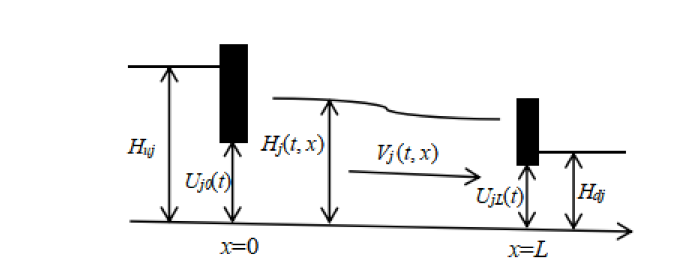
其中, Hdi 和 Huj 表示该渠道下游 (down) 和上游 (up) 的水位高度 (如图2所示).
图2
并且, 在星形渠道连接点处的流量关系表达式为
(2.5) 式表明, 第 n 段渠道作为出口通道, 其左边界是不能作为控制端的, 其动力学由流量守恒关系所约束. 另外, 设系统的平衡状态为 H∗i,V∗i, 且需满足
∙ gH∗i>(V∗i)2 (亚临界流动条件),
∙ Huj>H∗j>Hdj,H∗n>Hdn,V∗i>0,
∙ H∗nV∗n=n−1∑j=1H∗jV∗j,
∙ SiH∗i=Ci(V∗i)2.
2.2 模型 (2.1) 的线性化
在这一部分, 采用黎曼坐标变换将系统 (2.1) 在平衡态附近进行线性化处理. 令
则系统 (2.1) 的线性化模型为如下特征形式
其中
2.3 边界条件及时滞控制器设计
同文献 [19] 单渠道模型的边界状态反馈控制器类似, 本文的控制律如下
其中, Rj1,Ri2 为任意常数, Uj(t) 表示动态反馈控制器.
同时, 由节点处的流量关系式 (2.5) 可得, 位于网络连接点处的边界条件为
其中, Rn1=λn2λn1,αj=λj1−Rj2λj2λn1.
本文考虑采用时滞动态反馈控制器
去镇定受控系统 (2.7)-(2.9), 且 Kjp,Kjd 代表反馈参数, τj>0 表示反馈时滞. 从而, 使系统 (2.1) 的状态达到平衡态 (H∗i,V∗i), 及 n−1 段入口通道的输出量测 yj0(t) 达到期望值 H∗j.
注 2.1 根据 (2.2)-(2.4), (2.6) 和 (2.8) 式, 计算可得边界上自适应控制闸门开度
显然, 由 (2.2) 和 (2.11) 式可以看出, 要实现输入控制 UiL 和 Uj0, 只需要在线量测 2n−1 个边界水位高度 Hj0 和 HiL 即可. 这一结果在工程水动力学实践中具有重要意义, 因为在实际应用中测量渠道流量是十分困难的.
2.4 系统重构
令
则时滞系统 (2.7)-(2.10) 可写为如下 PDE-PDE 无穷维耦合系统的形式
其中
3 闭环系统稳定性分析
本节我们的目标是构造一个合适的加权 Lyapunov 函数去分析闭环系统 (2.13) 的指数稳定性.
首先, 考虑构造如下的 Lyapunov 候选函数
其中
且 pj1,pj2,pj3,pj4,q,μi 为待定正常数.
其次, 利用分部积分公式和 (2.13) 式中的边界条件, 对 (3.1) 式沿时间 t 求导数.
步骤 1 将 (3.2) 式对时间 t 求导数, 得
其中
且
将 (2.13) 式中的边界条件代入 (3.5) 式得
于是, ˙Vj1(t)≤0 等价于
此外, \dot{V}_{j2}(t)<0 为负定二次型当且仅当
即
显然, 条件 (3.10)(a) 恒成立. 对于 (3.10)(b) 式, 考虑到
故若选取 \delta_j p_{j1}=\gamma_j p_{j2}, 且 \mu_j>0 充分小, 则条件 (3.10)(b) 亦可保证.
步骤 2 分析 V_n(t) 沿着系统 (2.13) 的解对时间 t 的导数.
其中 \zeta=\min\big\{\frac{\lambda_{n1}\mu_n}{2},\frac{\lambda_{n2}\mu_n}{2}\big\},
同前类似可证, 若选取参数 q 满足 q\delta_n=\gamma_n, 且 \mu_n>0 充分小, 则 \Omega 为正定矩阵.
最后, 令参数 q 满足
则结合 (3.4)-(3.12) 式易得, 必存在 \nu>0 使得
综上分析可得本文主要结论.
定理 3.1 设参数 k_{i0}\neq0,\;k_{i2}\neq0\ (i=1,2,\cdots,n). 闭环系统 (2.13) 指数稳定, 如果存在正实数 p_{jl}\ (j=1,2,\cdots,n-1,\;l=1,2,3,4)、q 以及充分小的 \mu_i>0 使得系统参数和时滞值 \tau_j>0 满足
注 3.1 结合 (2.2) 和 (2.6) 式计算可得
因此, 当系统 (2.13) 的状态 \xi_{i1}(t,x) 和 \xi_{i2}(t,x) 收敛到 0 时, 这 2n-1 个在线输出量测调控到指定参考信号 H_i^*.
4 数值模拟
本节旨在用数值仿真例子来说明时滞控制器对星形渠道网络系统 (2.7) 的镇定作用. 选取参数如下: 渠道段数 n=3, 渠道长度 L_i=1000 m, 宽度W_i=20 m, 底面坡度 S_i=0.0018, 摩擦系数 C_i=0.001 s^2/m, 稳态流率 Q_i^*=300 m^3/s. 利用稳态关系
可以计算稳态水深和流率分别为 H_i^*=5 m, V_i^*=3 m/s 以及系统 (2.7) 中的参数分别是
令
且
因此, 由定理 3.1 中的条件 (3.14) 可知, 如果反馈参数满足
则星形渠道网络系统 (2.13) 的指数稳定性是可以保证的. 图3 和图4 展示了系统 (2.13) 出口通道状态的收敛性, 其调控参数取值分别为 k_{j0}=k_{j1}=0.1\ (j=1,2),\;k_{32}=0.3, 初始条件为 \xi_{31}(0,x)=\cos(2\pi x)-\frac{1}{2},\;\xi_{32}(0,x)=\sin(2\pi x)+\frac{1}{2}. 取边界反馈系数 R_{11}=R_{21}=0.05, 由 (2.14) 式计算可得 K_{jp}=-0.156,\;K_{jd}=0.296\ (j=1,2). 图5 展示了 PDP 控制器 U_j(t)=K_{jp}(H_j(t,0)-H_j^*)+K_{jd}(H_j(t-\tau_j,0)-H_j^*) 的稳定性. 此外, 图6 表明, 入口通道的输出量测 y_{j0}(t) 调控到了期望参考值 H_{j}^*.
图3
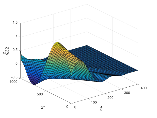
图4
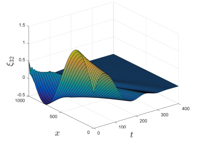
图5
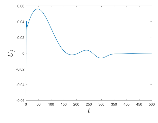
图6
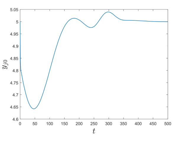
注 4.1 从条件 (3.14) 可以看出, 控制器中时滞参数值的范围无法显式表达. 但是, 若系统参数及反馈参数的取值如上, 则计算可得时滞 \tau_j 的范围为 0.38\leq\tau_j\leq4.35.
5 结论
本文讨论了星形网络渠道系统的时滞控制器设计与指数稳定性分析, 是对文献 [19] 单渠道模型的推广. 该星形网络包含 n 个子系统: 前 n-1 条入口通道并联流入多纽结, 后1条出口通道从结点处流出. 星形明渠网络系统边界反馈控制的目标是, 对于给定的平衡态, 结合在线量测得到的 2n-1 个边界水位高度, 实现边界上闸门开度的自适应控制. 考虑到明渠河流传播过程中存在时间延迟, 在入口通道边界上采用时滞动态反馈控制器去镇定受控系统, 并利用 Lyapunov 函数方法建立了闭环系统的指数稳定性, 给出了有关控制参数和时滞值的显式充分耗散条件. 下一步的研究工作是建立树形明渠网络系统的边界反馈控制律和自适应控制闸门开度, 研究闭环系统的指数稳定性.
参考文献
Experimental validation of a methodology to control irrigation canals based on Saint-Venant equations
DOI:10.1016/j.conengprac.2004.12.010 URL [本文引用: 1]
Boundary control of open channels with numerical and experimental validations
DOI:10.1109/TCST.2008.919418 URL [本文引用: 1]
On Lyapunov stability of linearised Saint-Venant equations for a sloping channel
DOI:10.3934/nhm.2009.4.177 URL [本文引用: 2]
Boundary feedback control in networks of open channels
DOI:10.1016/S0005-1098(03)00109-2 URL [本文引用: 1]
A Lyapunov approach for the control of multi reach channels modelled by Saint-Venant equations
Boundary PI controllers for a star-shaped network of 2\times2 systems governed by hyperbolic partial differential equations
Output regulation for a cascaded network of 2\times2 hyperbolic systems with PI controller
DOI:10.1016/j.automatica.2018.01.010 URL [本文引用: 1]
The spectral analysis and exponential stability of a 1-d 2\times2 hyperbolic system with proportional feedback control
A quadratic Lyapunov function for Saint-Venant equations with arbitrary friction and space-varying slope
DOI:10.1016/j.automatica.2018.10.035 URL [本文引用: 1]
Analog study of dead-beat posicast control
DOI:10.1109/TAC.1958.1104844 URL [本文引用: 1]
时滞反馈控制的若干问题
Some problems of delayed feedback control
Stabilization of linear undamped systems via position and delayed position feedbacks
DOI:10.1016/j.jsv.2007.11.001 URL [本文引用: 1]
Exponential stability and spectral analysis of the pendulum system under position and delayed position feedbacks
DOI:10.1080/00207179.2011.582886 URL [本文引用: 1]
Exponential stability and spectral analysis of the inverted pendulum system under two delayed position feedbacks
DOI:10.1007/s10883-012-9143-6 URL [本文引用: 1]
Balancing the inverted pendulum using position feedback
Time-Delayed feedback control of a hydraulic model governed by a diffusive wave system
一类扩散波方程的PDP反馈控制和稳定性分析
The PDP feedback control and stability analysis of a diffusive wave equation
