

1 引言
其中, Ω 是 RN(N>1) 中具有光滑边界 ∂Ω 的有界开区域, ν 是 ∂Ω 上的单位法向量, U(x,t), V(x,t) 代表时间 t>0 和空间位置 x∈Ω 时活化剂和抑制剂的浓度, 参数 DU 和 DV 表示活化剂和抑制剂的扩散系数, α0α, ρ 表示源浓度, r 和 γ 表示分解系数, κ, c′ 是与活化剂和抑制剂结果相关的系数, Um,Ul,Vn, 和 Vk 是 U 和 V 的功率, 分别用于测量自催化和交叉催化引起的活化剂和抑制剂的产生和破坏. Gierer 和 Meinhardt[3]证明了在适当的条件下, 活化抑制反应扩散模型能够产生空间斑纹. 至此, Gierer-Meinhardt 模型被经常用来描述形态的形成以及斑图的形成机制, 参见文献 [4⇓-6].
基于模型(1.1), 一些数学模型相继提出, 且已经有了很多结论. 以往的研究中, 针对模型 (1.1) 考虑了两种情形: (i) 当 m=2,n=1,l=2,k=0 时, Miura 和 Maini[7]利用线性稳定性分析, 得到了模型中特定参数的微小变化能够影响图灵斑图出现的速度. 接着, Gonpot 和 Colet[8]通过非线性分支分析, 研究了扩散和 Turing 不稳定性在活化抑制模型中对图形形成的作用. 进一步, Song 等[9]研究了模型的 Turing-Hopf 分支和空间共振现象, 为更好理解模型在分支点附近的动力学行为, 提出了二维空间共振分支规范型计算的一般方法. 最近, 杨等[10]对模型进行无量纲化, 研究了正常数平衡解的 Turing 不稳定性和空间周期解问题. 同时, 还采用了较多的数值模拟方法, 对理论结果进行了进一步验证. 另外, Liu 等[11]研究了这类模型在非齐次 Dirichlet 边值条件下系统的 Hopf 分支以及稳态分支, 得到了空间上的非均匀周期解和非常数正稳态解; (ii) 当 m=2,n=2, l=1,k=0 时, Wang 等[12]研究了这类模型在齐次 Neumann 边界条件下的 Turing 不稳定性和 Hopf 分支.
情况 (i) 和 (ii) 表明, Gierer-Meinhardt 活化抑制模型 (1.1) 已进行了广泛的研究, 为了更好地理解模型 (1.1) 的动力学行为, 如下考虑 m=2,n=1,l=2 和 k=0 所对应 Gierer-Meinhardt 活化抑制模型
其中参数 b,d 都是正实数.
现实生活中的一些问题可能取决于扩散[13⇓-15], 但也往往取决于时间[16], 为了修正依赖于系统过去历史的模型动力学行为, 建立具有生物学意义的数学模型, 还需考虑时滞效应. 而在时滞反应扩散系统中, 从时间和空间两个方面刻划客观事物可以更准确地描述生物种群的变化规律[17]. Lee[18]认为在这一描述生物现象的化学反应中活化剂和抑制剂分子受到基因表达时滞的影响, 因此基于模型(1.1) 提出了具时滞及具饱和项和时滞的 Gierer-Meinhardt 模型. 近年来, 时滞对于化学反应模型的影响得到了更多学者的关注, 参见文献 [19⇓⇓⇓-23]. 受此启发, 本文拟讨论如下具有时滞的活化抑制模型
系统 (1.2) 有一正平衡点 (1b,1b2), 且当 0<b<1 时, 正平衡点 (1b,1b2) 是局部渐近稳定的, 即系统 (1.3) τ=0 时的结论. 本文讨论了一类 Gierer-Meinhardt 活化抑制模型中时滞 τ 对正平衡点 (1b,1b2) 稳定性的影响. 特别地, 对于定义在 0<b<1 上的函数 τjn(b), 证明了τjn(b) 关于 n, j 分别是严格单调递增的, τjn(b) 关于 b 是严格单调递减的, 进一步,
因此, 当τ<τ00(b) 时, 正平衡点 (1b,1b2) 是局部渐近稳定的; 当 τ>τ00(b) 时, 正平衡点 (1b,1b2) 是不稳定的; 此外, 当 τ=τ00(b) 时, 系统 (1.3) 在正平衡点 (1b,1b2) 处产生 Hopf 分支, 即表示系统的平衡 (或稳定状态) 经历稳定且周期性的振荡变化.
从生物学的角度来看, Hopf 分支的出现意味着时滞能够调节细胞激活和抑制的过程, 并影响生物系统中的信号传递速度, 从而引发或改变细胞之间的相互作用模式. 此外, 时滞 τ 能够影响系统的稳定性, 在 Hopf 分支出现之前, 系统往往是稳定的; 然而, 当时滞达到一定阈值时, 系统可能会失去稳定性转变为振荡状态. 这种转变导致生物体内部的变化和适应, 对于细胞分化, 组织形态调控等过程具有重要意义.
本文主要证明了下面的结果, 即当时滞 τ 发生变化时, 对模型 (1.3) 正平衡点的稳定性, 分支的存在性, 分支方向和周期解稳定性的影响.
定理 1.1 假设 d,l 都是正常数, 且 d>1, 令 0<b<1, 则
(1) 若系统 (1.3) 存在一临界值 τ00(b), 当 τ<τ00(b), 正平衡点 (1b,1b2) 是渐近稳定的; 当 τ>τ00(b), 正平衡点 (1b,1b2) 是不稳定的; 特别地, 当 τ=τ00(b), 系统 (1.3) 在正平衡点 (1b,1b2) 处发生 Hopf 分支.
(2) 记 μ2 表示分支方向, β2 表示分支周期解的稳定性: 若 μ2>0(<0), 则分支方向为向前 (向后), 且当 τ>τ00 (<τ00) 存在周期解; 若 β2<0(>0), 则分支周期解是渐近稳定的 (不稳定的).
全文安排如下, 在第 2 节中, 通过研究特征方程, 分析了系统 (1.3) 正平衡点的稳定性, 并表明在正平衡点 (1b,1b2) 处发生 Hopf 分支; 第 3 节, 利用中心流形定理和正规型理论研究分支方向和分支周期解的稳定性; 最后证明了在时滞取某个临界值时系统存在 Hopf 分支, 并利用数值模拟验证理论结果.
2 平衡点的稳定性与分支的存在性
本节在有界区域 Ω=(0,lπ),l∈R+ 上考虑系统
首先, 系统 (2.1) 有唯一的正平衡点 (1b,1b2), 下面讨论正平衡点 (1b,1b2) 的稳定性. 通过变换 ˆu=u−1b, ˆv=v−1b2, 将平衡点 (1b,1b2) 平移到原点 (0,0), 为方便起见, 仍记 ˆu, ˆv 为 u, v. 于是系统 (2.1) 变为
其中 u=u(x,t), uτ=u(x,t−τ), v=v(x,t). 定义 X=C([lπ],R2). 在抽象空间 C([−τ,0],X) 中, 系统 (2.2) 可以写成以下抽象的泛函微分方程
这里,dΔ=(Δ,dΔ),dom(dΔ)={(u,v)T:u,v∈C2([lπ],R),ux=vx=0,x=0,lπ},且 L:C([−τ,0],X)→X,F:C([−τ,0],X)→X,根据系统 (2.2) 有
其中 ϕ=(ϕ1,ϕ2)T∈C([−τ,0],X),
于是系统 (2.2) 在平衡点 (1b,1b2) 处的线性化可写为
根据文献 [25], 其线性部分对应的特征方程是
由特征值问题 −ψ″ 有 \mu_{n}=\frac{n^{2}}{l^{2}}\ (n=0,1,2,\cdots ), 相应的特征函数 \psi_{n}(x)=\cos\frac{n}{l}x, 从而
将 y 的表达式代入特征方程 (2.5) 化简可得
根据特征方程 (2.5) 知
其中
若 \lambda=\pm {\rm i}\sigma(\sigma>0) 是 (2.6) 式的一对纯虚根, 则
由上述计算化简可得
其中
因为对于任意的 0<b<1, 都有 \lim\limits_{n\rightarrow 0}(B_{n}^{2}-C^{2})<0, \lim\limits_{n\rightarrow\infty}(B_{n}^{2}-C^{2})=+\infty, 所以存在最小的 N_{0}(b)\geq0, 使得当 n>N_{0} 时等式 (2.8) 没有正根, 当 0 \leq n \leq N_{0} 时等式 (2.8) 至多有一个正根.
且当
等式 (2.6) 有一对纯虚根 \pm {\rm i}\sigma, 其中 \tau_{n}^{0} 满足
这里令 N=\max\limits_{0<b<1}N_0(b), 下面讨论曲线 \tau=\tau_n^j(b)\ (0\leq n\leq N, j\in \mathbb{N}_0) 的有关性质.
引理 2.1 设 D_n 为 \tau=\tau_n^j(b)\ (0 \leq n \leq N, j\in \mathbb{N}_0) 的定义域, 因此
证 从 (2.13) 式中, 易知 \tau_n^0(b) 是等式 (2.6) 有一对纯虚根的最小正 \tau 值, 且当 (2.8) 式有一正根时, 等式 (2.6) 有一对纯虚根. 因为 A_{n}^{2}-2B_{n} 总是非负的, 那么 (2.6) 式有一对纯虚根当且仅当 B_{n}^{2}-C^{2}<0. 于是可以得到 \tau_n^0(b) 的定义域是
因为 \tau_n^j(b)\ (j\geq 1) 和 \tau_n^0(b) 有相同的定义域, 所以 D_n 也是 \tau_n^j(b)\ (j\geq 1) 的定义域.
令 \lambda_{n}(\tau)=\gamma_{n}(\tau)+{\rm i}\sigma_{n}(\tau) 是等式 (2.6) 的根, 且当 \tau\rightarrow\tau_{n}^{j} 时, 有 \gamma_{n}(\tau_{n}^{j})=0, \sigma_{n}(\tau_{n}^{j})=\sigma_{n}. 于是横截条件如下.
引理 2.2 \gamma_{n}'(\tau_{n}^{j}(b))>0, 其中 b\in D_n, 0\leq n\leq N, j\in \mathbb{N}_0.
证 将 \lambda_{n}(\tau) 代入等式 (2.6) 并关于 \tau 求导有
因为 \sigma_n 和 \tau_{n}^{j} 满足 \sigma^{2}-B_{n}=C\cos\sigma\tau 和 \sigma A_{n}=C\sin\sigma\tau, 则由 \sigma_n^2 的表达式可以得到
因此, \gamma_{n}'(\tau_{n}^{j})>0.
注 2.1 由上述可知, 当 0\leq n\leq N_0(b) 时, 满足 B_{n}^{2}-C^{2}<0, 由于此时 A_{n}^{2}-2B_{n} 关于 b 求导, B_{n}^{2}-C^{2} 关于 n, b 求导均较为复杂, 难于判断, 但若限制 l\sqrt{b}<n, 那么 A_{n}^{2}-2B_{n}, B_{n}^{2}-C^{2} 相关求导便容易看出, 如图1.
图1
此时取 b=0.5, d=2, l=5, 即当 l\sqrt{b}<n 时, 仍满足 B_{n}^{2}-C^{2}<0 成立. 因此下面考虑当 l\sqrt{b}<n\leq N_0(b) 时 \tau_{n}^{j}(b) 的相关性质.
从 (2.12) 式容易看出 \tau_{n}^{j+1}(b)>\tau_{n}^{j}(b). 又因为当 0<b<1 时, 有 A_n\geq0, 那么对于任意的 b\in D_n, 根据 (2.13) 式有
因此可以得到曲线 \tau_{n}^{j}(b) 的以下结论.
引理 2.3 假设 d>1, 当 0<b<1 时, 对于任意的 l\sqrt{b}<n\leq N_0(b), j\in\mathbb{N}_0, 都有 \tau_{n+1}^{j}(b)>\tau_{n}^{j}(b).
证 若 d>1, 根据 (2.11) 式,
其中 A_{n}^{2}-2B_{n} 和 B_{n}^{2}-C^{2} 分别由 (2.9) 和 (2.10) 式给出, 因为当 0<b<1, l\sqrt{b}<n\leq N_0(b) 时, A_{n}^{2}-2B_{n} 关于 n 严格单调递增, C^{2}-B_{n}^{2} 关于 n 严格单调递减, 所以 \sigma_{n+1}^2(b)<\sigma_n^2(b). 又由当 0<b<1 时, 有 A_n\geq0, 根据 (2.13) 式有 \tau_n^0=\frac{\arccos\frac{\sigma_{n}^{2}-B_{n}}{C}}{\sigma_{n}}, 从而 \tau_{n+1}^0(b)>\tau_n^0(b), l\sqrt{b}<n\leq N_0(b).
因为 \sigma_{n+1}<\sigma_n, 所以根据 (2.12) 式可得 \tau_{n+1}^{j}(b)>\tau_{n}^{j}(b), j\geq1, l\sqrt{b}<n\leq N_0(b).
引理 2.4 假设 d, l 是正常数, 定义 l_n=\big(\frac{(\sqrt{d^2-6d+1}+d-1)n^2}{2}\big)^{\frac{1}{2}}, n\in\mathbb{N}_0, 使得 \bigcup\limits_{n=0}^{\infty}(l_n, l_{n+1}]=\mathbb{R}^+. 那么对于任意的 l\in(l_n, l_{n+1}], 都存在 \{b_p\}_{p=0}^{n}, 使得 0=b_0<\cdot\cdot\cdot<b_{p}<b_{p+1}<\cdot\cdot\cdot<b_n 满足如下性质
(1) 若 l\sqrt{b}<p\leq n, 则 D_p=(b_p,1), 若 p>n, 则 D_p=0, 其中 N=\max\limits_{0<b<1}N_0(b)=n;
(2) 当 b\in (b_p,1), l\sqrt{b}<p\leq n, j\in \mathbb{N}_0, \tau_{p}^{j}(b) 关于 b 是严格单调递减函数;
(3) 对于 l\sqrt{b}<p\leq n, j\in \mathbb{N}_0, 有 \lim\limits_{b\rightarrow b_p}\tau_{p}^{j}(b)=+\infty, \lim\limits_{b\rightarrow 0}\tau_{p}^{0}(b)>0 和 \lim\limits_{b\rightarrow 1}\tau_{0}^{0}(b)=0.
证 当 0<b<1, p\in \mathbb{N}_0 时, B_{p}^{2}-C^{2} 关于 b 是严格单调递减的. 因为对于任意的 l\in (l_n, l_{n+1}], 当l\sqrt{b}<p\leq n 时, \lim\limits_{b\rightarrow 0}B_{p}^{2}-C^{2}<0, 当 p>n 时, \lim\limits_{b\rightarrow 0}B_{p}^{2}-C^{2}\geq 0, 那么存在 \{b_p\}_{p=0}^{n}, 使得 0=b_0<\cdot\cdot\cdot<b_{p}<b_{p+1}<\cdot\cdot\cdot<b_n 满足D_p=(b_p,1), l\sqrt{b}<p\leq n, 且 D_p =0, p>n, 其中 N=\max\limits_{0<b<1}N_0(b)=n.
下证 \tau_{p}^{0}(b) 关于 b 是严格单调递减的, 根据 (2.11) 式
且
因为 C^{2}-B_{p}^{2} 关于 b 是严格单调递增的, \frac{C^{2}-B_{p}^{2}}{C} 关于 b 是严格单调递增的, \frac{B_{p}}{C} 关于b 是严格单调递减的, 且 A_{p}^{2}-2B_{p} 关于 b 是严格单调递减的, 同时由上可得 \sigma_p 和 \frac{\sigma_p^2}{C} 关于b 是严格单调递增的, 那么根据 (2.15) 式可知, 当 b\in (b_p,1), l\sqrt{b}<p\leq n, j\in \mathbb{N}_0 时, \tau_{n}^{j}(b) 关于 b 是严格单调递减函数.
由于当 l\sqrt{b}<p\leq n 时, \lim\limits_{b\rightarrow b_p}\sigma_p(b)=0, \lim\limits_{b\rightarrow 1}\sigma_p(b)>0, 且 \lim\limits_{b\rightarrow 1}\arccos\frac{\sigma_0^2-B_0}{C}=0, 从而根据 (2.15) 式可得 \lim\limits_{b\rightarrow b_p}\tau_p^0(b)=+\infty, \lim\limits_{b\rightarrow 1}\tau_p^0(b)>0, 以及 \lim\limits_{b\rightarrow 1}\tau_0^0(b)=0.
定理 2.1 假设 d, l 都是正常数, 且 d>1, 那么当 0<b<1 时, 有
(1) 如果 \tau\in (0,\tau_{0}^{0}(b)), 那么方程 (2.+) 中的所有根都具有负实部, 从而正平衡点 \left(\frac{1}{b},\frac{1}{b^2}\right) 是局部渐近稳定的.
(2) 如果 \tau=\tau_{0}^{0}(b), 那么方程 (2.6) 的根除了 \pm {\rm i}\sigma_0 外, 其余都具有负实部, 且此时系统在正平衡点 \left(\frac{1}{b},\frac{1}{b^2}\right) 处经历 Hopf 分支.
(3) 如果 \tau>\tau_{0}^{0}(b), 那么正平衡点 \left(\frac{1}{b},\frac{1}{b^2}\right) 是不稳定的.
3 分支方向和周期解的稳定性
令 \tau=\tau_0+\mu, 由上一节分析可知 \mu=0 是系统 (2.3) 的 Hopf 分支值, 再令 \widetilde{t}=\frac{t}{\tau} 规范化时滞, 于是系统 (2.3) 变为
其中对于 \phi\in C([-1,0],X) 有
由第 2 节可知, \pm {\rm i}\sigma_0\tau_0 是线性系统的一对纯虚特征根, 因此有
其线性泛函微分方程为
应用 Riesz 表示定理可知, 存在一个有界变差 2\times2 矩阵函数 \eta(\theta,\mu)(\theta\in[-1,0]) 使得
事实上,
其中
对于任意的 \phi(\theta) \in C^1([-1,0],\mathbb{R}^{2}), 定义 A(0) 为
以及对于任意的 \psi=(\psi_{1},\psi_{2}) \in C^{1}([0,1],(\mathbb{R}^{2})^{*}), 定义
定义双线性函数
其中, A(0) 和 A^{*} 是正规伴随算子.
易证 \pm {\rm i}\sigma_0\tau_0 是 A(0) 和 A^{*} 的特征值,
分别是 A(0) 和 A^{*} 对应于特征值 {\rm i}\sigma_0\tau_0 和 - {\rm i}\sigma_0\tau_0 的特征向量, 其中
令 \Phi=(q(\theta),\overline{q}(\theta)), \Psi=(q^{*}(s),\overline{q}^{*}(s))^{T}, 那么 (\Phi,\Psi)_0=I, I=\left( \begin{array}{cc} 1 & 0 \\ 0 & 1 \end{array} \right).
进一步, 令 f_{0}=(f_{0}^{1},f_{0}^{2})^{T}, 其中f_{0}^{1}= \left( \begin{array}{c} 1 \\ 0 \end{array} \right) \notag, f_{0}^{2}= \left( \begin{array}{c} 0 \\ 1 \end{array} \right) \notag.
通过定义 c\cdot f_0=c_1\cdot f_0^1+c_2\cdot f_0^2, c=(c_1,c_2)^T\in\mathbb{C}^2, 在希尔伯特空间 X 上定义内积如下
这里 u=(u_{1},u_{2}), v=(v_{1},v_{2}) \in X=C([l\pi],\mathbb{R}^{2}), 并且对 \phi \in C([-1,0],X), 有
线性方程 (3.2) 在 \mu=0 时的中心子空间是 P_{CN}\mathcal{C}, 且
对 \mathcal{C} 进行空间分解, \mathcal{C}=P_{CN}\mathcal{C}+P_{S}\mathcal{C}, 其中 P_{S}\mathcal{C} 表示稳定子空间.
根据文献 [24] 可知, 线性系统 (2.3) 无穷小生成元 A_U 满足 A_U\psi=\dot{\psi}(\theta), 其中 \psi\in {\rm dom}(A_U), 当且仅当 \dot{\psi}(\theta)\in\mathcal{C}, \psi(0)\in {\rm dom}(\Delta) 有 \dot{\psi}(\theta)(0)=\tau_0\Delta\psi(0)+\tau_0L_0(\psi).
由于计算分支方向和分支周期解稳定性的公式都只和值 \mu=0 有关, 故令 (3.1) 式中 \mu=0, 得到如下中心流形
方程 (3.1) 在中心流形上的解半流可以写成
其中
即
这里
定义
将其泰勒展开有
O(4)=O(\|(u,v)\|^{4}), 根据 G(\phi,0)=\tau_{0}F_{0}(\phi)=\tau_{0}(G_{1},G_{2})^{T}, 那么
因此可以得出
如上表达式可以看出, 为了计算 g_{21}, 需要计算 W_{11}(\theta) 和 W_{20}(\theta).
因为 W(z(t),\bar{z}(t)) 满足
根据
可得
当 \theta \in [-1,0) 时,
于是结合 (3.10) 和 (3.15) 式有
联立 (3.15) 式的第一个方程和 (3.16) 式可得
再联立 (3.15) 式的第二个方程和 (3.17) 式可得
取 (3.15) 式中 \theta=0, 利用 A_U 的定义和
分别得到
其中
综上, g_{21} 可计算得到.
基于以上分析看出, 每个 g_{ij} 都能通过参数确定, 因此可以计算以下量来决定分支方向和分支周期解的稳定性
定理 3.1 根据系统 (2.1) 有如下结论.
(1) \mu_2 决定 Hopf 分支的分支方向: 若 \mu_2>0(<0), 则当 \tau>\tau_0=\tau_0^0(<\tau_0=\tau_0^0) 存在周期解, 即分支方向为向前 (向后);
(2) \beta_2 确定分支周期解的稳定性: 若 \beta_2<0(>0), 则分支周期解是渐近稳定的 (不稳定的);
(3) T_2 决定分支周期解的周期变化: 若 T_2>0(<0), 则周期增大 (减小).
4 数值模拟
基于上述分析, 下面将使用空间离散有限差分法数值求解系统 (2.1) 在区间 \Omega=(0,3\pi) 上的动力学现象.
取参数 d=2, b=0.5, 此时研究时滞对系统 (2.1) 动力学行为的影响. 通过计算得到 \tau_0^0=0.5097, \sigma_0=0.6656, Re(C_1(0))=-2.5809<0, 同时有, \mu_2=1.2083>0, Hopf 分支方向是超临界的; \beta_2=-5.1618<0, Hopf 分支周期解是渐近稳定的; T_2=-0.6056<0, Hopf 分支周期解的周期减少.
由于文中的理论部分主要关注系统 (2.1) 的分析和推导, 然而在实际的数值模拟过程中发现, 将系统 (2.1) 的 ODE 系统作为一个关联问题纳入研究是有意义的. ODE 系统在某些情况下可以提供与 PDE 系统相关的重要信息, 并对其结果进行验证和补充. 因此, 模拟如下
图2
图2
当参数 \tau=0.42<\tau_0^0 时, 初值: (u_{0},v_{0})=(1.8, 4.2), 系统 (2.1) 的 ODE 系统在正平衡点 (2,4) 是稳定的
图3
图3
当参数 \tau=0.51>\tau_0^0 时, 初值: (u_{0},v_{0})=(1.8, 4.2), 系统 (2.1) 的 ODE 系统在正平衡点 (2,4) 是不稳定的
图4
图4
当参数 \tau=0.42<\tau_0^0=0.5097 时, 初值: (u_{0}(x),v_{0}(x))=(2+0.5\sin(4.5x), 4-0.5\sin(4.5x), 系统 (2.1) 的解收敛到常值稳态解 (2,4)
图5
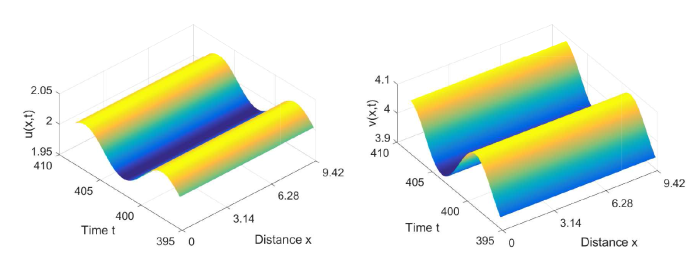
图5
当 \tau=0.51>\tau_0^0=0.5097, 初值: (u_{0}(x), v_{0}(x))=(2+0.5\cos(2x),4-0.5\cos(2x)), 系统 (2.1) 的解收敛到空间齐次的周期解
图6
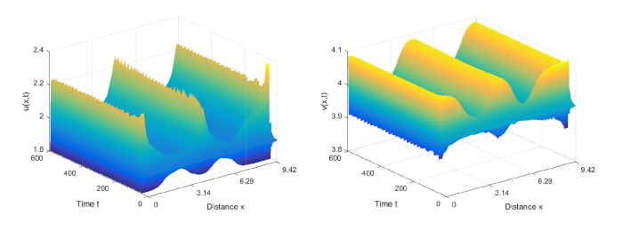
图6
当 \tau=0.51>\tau_0^0=0.5097, 初值: (u_{0}(x), v_{0}(x))=(2+0.1\cos(5x),4-0.1\cos(5x)), 系统 (2.1) 的解收敛到空间非齐次的周期解
参考文献
A theory of biological pattern formation
Application of a theory of biological pattern formation based on lateral inhibition
DOI:10.1242/jcs.15.2.321 PMID:4859215 [本文引用: 1]
Generation and regeneration of sequence of structures during morphogenesis
Spikes for the Gierer-Meinhardt system in two dimensions: The strong coupling case
DOI:10.1006/jdeq.2001.4019 URL [本文引用: 1]
The dynamics of a kinetic activator-inhibitor system
DOI:10.1016/j.jde.2006.03.011 URL [本文引用: 1]
Speed of pattern appearance in reaction-diffusion models: Implications in the pattern formation of limb bud mesenchyme cells
DOI:10.1016/j.bulm.2003.09.009 URL [本文引用: 1]
Gierer-Meinhardt model: Bifurcation analysis and pattern formation
DOI:10.3923/tasr.2008.115.128 URL [本文引用: 1]
Spatial resonance and Turing-Hopf bifurcations in the Gierer-Meinhardt model
DOI:10.1016/j.nonrwa.2016.02.006 URL [本文引用: 1]
空间齐次和非齐次下活化-抑制模型动力学分析
Dynamics analysis of activation-inhibition models under spatial homogeneous and heterogeneou
Multiple bifurcation analysis and spatiotemporal patterns in a 1-D Gierer-Meinhardt model of morphogenesis
DOI:10.1142/S0218127410026289
URL
[本文引用: 1]

A reaction–diffusion Gierer–Meinhardt model of morphogenesis subject to Dirichlet fixed boundary condition in the one-dimensional spatial domain is considered. We perform a detailed Hopf bifurcation analysis and steady state bifurcation analysis to the system. Our results suggest the existence of spatially nonhomogenous periodic orbits and nonconstant positive steady state solutions, which imply the possibility of complex spatiotemporal patterns of the system. Numerical simulations are carried out to support our theoretical analysis.
Stripe and spot patterns in a Gierer Meinhardt activator-inhibitor model with different sources
Global bifurcation analysis and pattern formation in homogeneous diffusive predator-prey systems
DOI:10.1016/j.jde.2015.10.036 URL [本文引用: 1]
Diffusion-Driven instability and bifurcation in the Lengyel-Epstein system
DOI:10.1016/j.nonrwa.2007.02.005 URL [本文引用: 1]
Effects of seasonal growth on ratio dependent delayed prey predator system
DOI:10.1016/j.cnsns.2007.10.013 URL [本文引用: 1]
Spatiotemporal dynamics of a leslie-gower predator-prey model incorporating a prey refuge
DOI:10.1016/j.nonrwa.2011.02.011 URL [本文引用: 1]
The influence of gene expression time delays on Gierer-Meinhardt pattern formation systems
DOI:10.1007/s11538-010-9532-5 URL [本文引用: 1]
Effects of delay in a reaction-diffusion system under the influence of an electric field
DOI:10.1103/PhysRevE.77.036202 URL [本文引用: 1]
Control of the Hopf-turing transition by time-delayed global feedback in a reaction-diffusion System
DOI:10.1103/PhysRevE.84.016222 URL [本文引用: 1]
Reaction-Cattaneo systems with fluctuating relaxation time
DOI:10.1103/PhysRevE.81.026205 URL [本文引用: 1]
Control of spatiotemporal patterns in the Gray-Scott model
DOI:10.1063/1.3270048
URL
[本文引用: 1]
This paper studies the effects of a time-delayed feedback control on the appearance and development of spatiotemporal patterns in a reaction-diffusion system. Different types of control schemes are investigated, including single-species, diagonal, and mixed control. This approach helps to unveil different dynamical regimes, which arise from chaotic state or from traveling waves. In the case of spatiotemporal chaos, the control can either stabilize uniform steady states or lead to bistability between a trivial steady state and a propagating traveling wave. Furthermore, when the basic state is a stable traveling pulse, the control is able to advance stationary Turing patterns or yield the above-mentioned bistability regime. In each case, the stability boundary is found in the parameter space of the control strength and the time delay, and numerical simulations suggest that diagonal control fails to control the spatiotemporal chaos.
Time-Delay-Induced instabilities in reaction diffusion systems
DOI:10.1103/PhysRevE.80.046212 URL [本文引用: 1]
Stability analysis of the Gierer-Meinhardt system with activator degradation
Stability and bifurcation of a delayed reaction-diffusion model with robin boundary condition in heterogeneous environment
DOI:10.1142/S0218127423500189
URL
[本文引用: 2]
In this paper, we investigate a reaction–diffusion model with delay and Robin boundary condition in heterogeneous environment. The existence, multiplicity and stability of spatially nonhomogeneous steady-state solutions and periodic solutions are studied by employing the Lyapunov–Schmidt reduction method. Moreover, the Hopf bifurcation direction is derived. It is observed that Robin boundary condition plays a crucial role in the Hopf bifurcation. More precisely, when the boundary effect is stronger than the interaction of the species within the region, there is no Hopf bifurcation no matter how the time delay [Formula: see text] changes. Finally, we illustrate our general theoretical results by an application to the Nicholson’s blowflies model.
Hopf bifurcation in a two-species reaction-diffusion-advection competitive model with nonlocal delay
Hopf bifurcation of a delayed reaction-diffusion model with advection term
一类具有时滞的营养-微生物扩散模型的 Hopf 分支研究
Hopf bifurcation of a nutritional microbial diffusion model with time delay
Hopf bifurcation in a reaction-diffusion model with Degn-Harrison reaction scheme
DOI:10.1016/j.nonrwa.2016.07.002 URL [本文引用: 1]
Center manifolds for partial differential equations with delay
