

1 引言
在早期实验中, 玻色子在磁势阱中不能发生自旋. 1998 年, 利用光学偶极子阱, 人们首次在自旋
在平均场意义下, 温度
初始条件
其中
这里
其中
这里
波函数
质量守恒
磁场量守恒
单个粒子能量守恒
其中
其中
基态模拟是 BEC 研究的重要问题. 自旋轨道耦合 Spin-2 BEC 的基态
其中非凸集
对于自旋轨道耦合旋量 BEC 模型, Yuan 等[23] 提出了投影梯度流法计算自旋轨道耦合 Spin-1 BEC 的基态. 该方法采用空间二阶有限差分和时间 Grank-Nicolson 方法离散连续梯度流, 具有总质量、总磁场量守恒及能量递减的性质. 然而, 自旋轨道耦合 Spin-2 BEC 模型具有复杂的自旋交换项和自旋单线态项, 其基态解在自旋轨道耦合效应下具有复杂的基态相, 可呈现细密的条纹状和晶格状两种图案. 这些特点对模拟自旋轨道耦合 Spin-2 BEC 基态的数值算法在精度与效率方面提出了新的挑战. 目前, 关于自旋轨道耦合 Spin-2 BEC 基态模拟的数值结果十分有限. 本文将带拉格朗日乘子的梯度流算法[11,17] 推广到自旋轨道耦合 Spin-2 BEC 的基态模拟. 该方法在每步迭代只需求解一个常系数椭圆方程(组), 易实施且效率高.
本文结构安排如下: 第 2 节介绍带拉格朗日乘子的正规梯度法, 给出该方法的梯度流方程及其投影系数的确定方法; 第 3 节介绍其离散格式; 第 4 节给出数值结果.
2 带拉格朗日乘子的正规梯度流法
自旋轨道耦合 Spin-2 BEC (1.1)-(1.3) 对应的连续正规梯度流 (CNGF) 定义为
这里
联立 (2.1)-(2.3) 式并以
其中
这里及下文, 如无特殊说明, 范数
易知连续正规梯度流 (2.1)-(2.3) 式具有总质量守恒、总磁场量守恒和能量稳定性, 但由于其为非线性积分方程组, 直接离散求解往往计算量大. 为避免这一困难, 下面考虑其一阶分裂格式导出的 GFLM. 取时间步长
投影步骤为
这里
其中
这里
因此, 为唯一确定所有投影系数
将 (2.11) 式代入 (2.10) 式, 易得关于
其中
直接计算可得
若假设至少有两个分量函数
进而由 (2.11) 式得
3 离散格式
在势函数
将有界区域
设
其中
稳定项因子
这里
通过对
这里
通过对 (3.1) 式的两边作快速傅里叶变换可得
化简得
通过对 (3.7) 式作逆快速傅里叶变换即得方程 (3.1) 的解.
4 数值实验
本章运用 GFLM 方法模拟自旋轨道耦合 Spin-2 BEC 在各参数下的基态. 对循环型体系
其中
的基态或其近似
算例 1 (可行性测试) 取
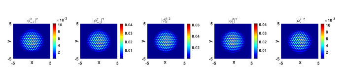
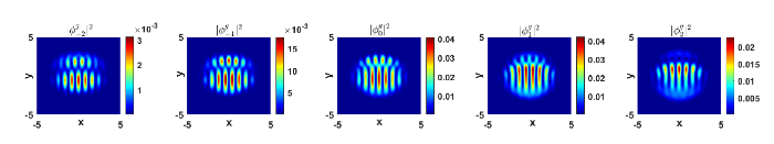
图1 是 GFLM 方法模拟算例 1 基态解的结果. 观察可得: (1) 基态解分量
图1
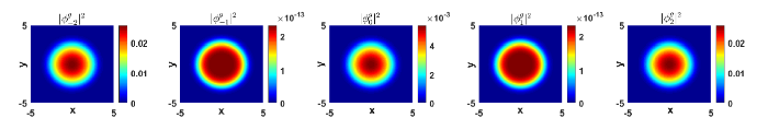
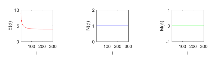
图2 表示计算过程中, 能量、总质量和总磁场量随迭代次数的变化情况. 观察可知: (1) 能量一直减少, 最后达到稳定状态; (2) 总质量
图2
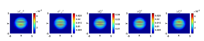
算例 2 (循环型体系下结果) 取
图3

图4

图5
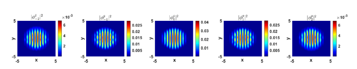
图6
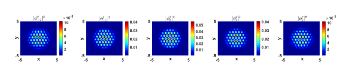
图7
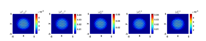
图8
算例 3 (循环型体系下结果) 固定
图9

图10
由上可得: GFLM 方法可以有效模拟循环型体系下自旋轨道耦合 Spin-2 BEC 的基态解; 磁场量
算例 4 (铁磁体系下结果) 取
图11
图12
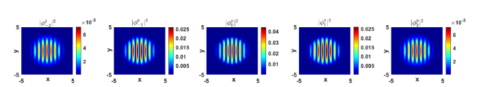
图13
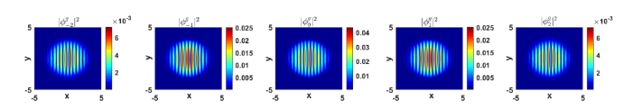
图14
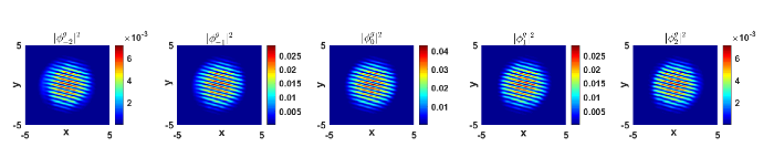
图15

图16
算例 5 (铁磁体系下结果) 固定
图17

图18
由上可得: GFLM 方法可有效模拟铁磁体系下自旋轨道耦合 Spin-2 BEC 的基态解; 磁场量
参考文献
Observation of Bose-Einstein condensation in a dilute atomic vapor

A Bose-Einstein condensate was produced in a vapor of rubidium-87 atoms that was confined by magnetic fields and evaporatively cooled. The condensate fraction first appeared near a temperature of 170 nanokelvin and a number density of 2.5 x 10(12) per cubic centimeter and could be preserved for more than 15 seconds. Three primary signatures of Bose-Einstein condensation were seen. (i) On top of a broad thermal velocity distribution, a narrow peak appeared that was centered at zero velocity. (ii) The fraction of the atoms that were in this low-velocity peak increased abruptly as the sample temperature was lowered. (iii) The peak exhibited a nonthermal, anisotropic velocity distribution expected of the minimum-energy quantum state of the magnetic trap in contrast to the isotropic, thermal velocity distribution observed in the broad uncondensed fraction.
Efficient spectral computation of the stationary states of rotating Bose-Einstein condensates by preconditioned nonlinear conjugate gradient methods
Mathematical models and numerical methods for spinor Bose-Einstein condensates
Computing the ground state solution of Bose-Einstein condensates by a normalized gradient flow
DOI:10.1137/S1064827503422956 URL [本文引用: 1]
Computing ground states of spin-1 Bose-Einstein condensates by the normalized gradient flow
DOI:10.1137/070698488 URL [本文引用: 1]
Ground state solution of Bose-Einstein condensate by directly minimizing the energy functional
DOI:10.1016/S0021-9991(03)00097-4 URL [本文引用: 1]
A mass and magnetization conservervative and energy-diminishing numerical method for computing ground state of spin-1 Bose-Einstein condensates
DOI:10.1137/070681624 URL [本文引用: 1]
Ground, symmetric and central vortex states in rotating Bose-Einstein condensates
DOI:10.4310/CMS.2005.v3.n1.a5 URL [本文引用: 1]
Plancks gesetz und lichtquantenhypothese
DOI:10.1007/BF01327326 URL [本文引用: 1]
Evidence of Bose-Einstein condensation in an atomic gas with attractive interaction
Efficient and accurate gradient flow methods for computing ground states of spinor Bose-Einstein condensates
DOI:10.1016/j.jcp.2021.110183 URL [本文引用: 3]
Bose-Einstein condensation in a gas of sodium atoms
Quantentheorie des einatomigen idealen gases
Quantentheorie des einatomigen idealen gases, zweite abhandlung
Spinor Bose condensates in optical traps
DOI:10.1103/PhysRevLett.81.742 URL [本文引用: 1]
Spinor Bose-Einstein condensates
DOI:10.1016/j.physrep.2012.07.005 URL [本文引用: 1]
Normalized gradient flow with Lagrange multiplier for computing ground states of Bose-Einstein condensates
DOI:10.1137/20M1328002 URL [本文引用: 2]
Synthetic magmetic fields for ultracold neutral stoms
DOI:10.1038/nature08609 [本文引用: 1]
Bose-Einstein condensates in a uniform light-induced vector potential
DOI:10.1103/PhysRevLett.102.130401 URL [本文引用: 1]
A spin-orbit-coupled Bose-Einstein condensates
DOI:10.1038/nature09887 [本文引用: 1]
Optical confinement of a Bose-Einstein condensate
DOI:10.1103/PhysRevLett.80.2027 URL [本文引用: 1]
Spinor Bose gases: Symmetries, magnetism, and quantum dynamics
DOI:10.1103/RevModPhys.85.1191 URL [本文引用: 1]
The numerical study of the ground states of spin-1 Bose-Einstein condensates with spin-orbit-coupling
DOI:10.4208/eajam URL [本文引用: 1]
