

1 引言
当疾病在某个地区出现时, 该地的疾病控制中心的首要任务就是竭尽全力防止疾病传播, 重要的预防措施之一就是通过大众传媒向人们普及正确的疾病预防知识. 在传染病传播的早期阶段, 媒体对传染病的报道能够加强公众的防范认识, 避免大众途经感染者停留的地方, 减少感染者的数量. 目前已经建立了一些数学模型研究媒体报道对传染病动力学影响[4,7,10,16,18,33,39,42]. 特别是Cui等[7]、 Caraballo等[4]、 Tchuenche等[32]、 Sun[31]等利用非线性函数f(I)=β−β1Ib+I研究媒体报道的影响, β代表在媒体报道之前, 接种者和感染者之间的接触率, 而β1代表在媒体报道后的最大降低接触率. 众所周知, 媒体的报道并不能完全阻止传染病的传播, 因此, β>β1的假设是合理的. 饱和发病率g(I)=I1+aI反映了感染者的行为变化和拥挤效应, a称为半饱和常数[11]. 当感染者数量较大时, g(I)会趋近于1a[1,3,21,25,26,28,30,34,35,38]. 文献[30]研究具有饱和发生率的传染病模型, 研究表明: 疫苗接种率提高使得感染者的密度降低. 其他发病率函数可以参考相关工作[6,13,14,17,19,24,27,36].
其中, S(t),V(t),I(t),R(t) 分别表示人群中t时刻易感者、接种者、感染者和恢复者的数量, γ 和K分别代表内禀增长率和环境最大容纳量; μ 表示自然死亡率; δ代表因病死亡率; τ表示感染者的恢复率; ρ表示易感者和感染者的接触率; θ 表示疫苗失效率; ζ 表示易感者接种疫苗率; a,b 都是半饱和常数; B1(t),B2(t),B3(t),B4(t)是相互独立的标准布朗运动; σ1,σ2,σ3,σ4表示白噪声的强度; (Ω,F,{Ft}t⩾是完备的概率空间, 且滤子\{\mathcal{F}_{t}\}_{t\geqslant 0}满足通常情况.
由于恢复者密度的变化不影响易感者、接种者和感染者的密度,所以模型(1.1)变换为
下面, 我们将证明模型(1.2)全局正解的存在唯一性, 寻找持久和遍历平稳分布存在的充分条件, 以及疾病灭绝的充分条件.
2 解的存在唯一性和持久性
模型(1.2)全局正解的存在性和唯一性是模型主要动力学性质之一. 对任意 t\geqslant0, 模型(1.2)的解记为\textbf{X}(t)=(S(t),V(t),I(t))^{\mbox{T}}. 定义 \mbox{d}\textbf{B}(t)=(\mbox{d}B_{1}(t), \mbox{d}B_{2}(t), \mbox{d}B_{3}(t))^{\mbox{T}}. 设\mathbb{R}^{n}是一个n维欧氏空间, X(t)是\mathbb{R}^{n}中的齐次马尔可夫过程, 则随机微分方程为
令初始值为 X(0) = X_{0}\in \mathbb{R}^{n}, g_{l}=(g^l_1,g^l_2,\cdots,g^l_n)^T 扩散矩阵为 A(X)=(a_{ij}(X))_{n\times n}, 其中 a_{ij}(X)=\sum\limits_{l=1}^{n}g_{l}^{i}(X)g_{l}^{j}(X). 定义随机微分方程的微分算子
定理2.1 对于任意初值(S(0), V(0), R(0))^{\mbox{T}}\in \mathbb{R}^3_+, 模型(1.2)存在唯一的正解, 且该解将以概率1留在\mathbb{R}^3_+ .
引理2.1 模型(1.2)的解\textbf{X}(t)具有以下性质
若 \max\{\sigma_{1}^{2}, \sigma_{2}^{2}, \sigma_{3}^{2}\}<2\mu, 则
定理2.2 若满足条件 {R}_{0}^{s}>1, \ \sigma_1^2<2(\gamma-\zeta), \ \max\{\sigma_{1}^{2}, \sigma_{2}^{2}, \sigma_{3}^{2}\}<2\mu, 则疾病是持久的, 且
证 构造如下C^2函数
其中c_1和c_2是待定正常数, 对V_{1} 应用Itô公式, 得到
并且
对V_{2}应用Itô公式, 得到
其中
定义V_{3}=V_{1}+3\sqrt [3] {c_{1}c_{2}(\beta-\beta_{1})\zeta K}V_{2}, 先对V_{3}应用Itô公式, 然后结合(2.3)和(2.5)式, 得到
根据(2.2)式, 令
因此
定义一个行向量\textbf{D}_1(t)和列向量 \mbox{d}\textbf{B}(t)=(\mbox{d}B_{1}(t), \mbox{d}B_{2}(t), \mbox{d}B_{3}(t))^{\mbox{T}}, 因此
对等式(2.8)两边同时积分, 再除以t, 结合(2.7)式得
其中
根据引理2.1和强大数定理[23] 可知\limsup\limits_{t\rightarrow\infty}\Psi_{1}(t) = 0, 对(2.9)式取下极限得\mathop{\liminf}\limits_{t\rightarrow\infty}A\langle I\rangle_{t}> \lambda>0. 证毕.
3 平稳分布的存在性
定理3.1 若{R}_{0}^{s}>1, 则模型(1.2)存在平稳分布, 并且具有遍历性.
证 定义有界集为
这里的\varepsilon 是非常小的正常数, 且满足以下条件
模型(1.2)扩散矩阵为
设模型(1.2)的扩散项最小值为
对任意的 \textbf{X}\in D_{\varepsilon}, \xi=(\xi_{1}, \xi_{2}, \xi_{3})^{\mbox{T}}\in \mathbb R_{+}^{3}, 都有
这意味着文献[5,注5.1]条件(i)已满足.
构造Lyapunov函数
其中
m>0 是充分小的常数满足
M>0 是充分大的常数满足
显然, W(\textbf{X}) 是连续函数, 所以存在最小值W(\bar{\textbf{X}}), 因此可构造非负的 C^{2} 函数
依次对V_{4}, V_{5}, V_{6} 应用 Itô 公式, 可得
其中
结合(2.7)式和(3.7)-(3.9)式, 我们得到
将\mathbb R_{+}^{3}\backslash D_{\varepsilon} 分成六个子区间, 证明 \mathcal{L}Q 在这六个区间内满足\mathcal{L}Q<-1, 其中\mathbb R_{+}^{3}\backslash D_{\varepsilon}=D_{1}\cup D_{2}\cup D_{3}\cup D_{4}\cup D_{5}\cup D_{6}.
情形 1 若\textbf{X}\in D_{1}, 则
根据(3.2), (3.5), (3.10)式, 可得
情形 2 若\textbf{X}\in D_{2}, 则
根据(3.2), (3.5), (3.10)式, 可得
情形 3 若\textbf{X}\in D_{3}, 则通过(3.3), (3.10)式可得
其中
情形 4 若 \textbf{X}\in D_{4}, 则通过(3.3), (3.10)式可得
情形 5 若\textbf{X}\in D_{5}, 则通过(3.3), (3.10)式可得
情形 6 若\textbf{X}\in D_{6}, 则通过(3.3), (3.10)式可得
所以文献[5,注5.1]条件(ii)已满足; 因此模型(1.2)存在遍历的平稳分布. 证毕.
4 疾病的灭绝性
定理4.1 若满足条件
则疾病将指数灭绝.
证 对模型(1.2) 的第一个方程两边同时从0到t 积分, 然后再除以t, 最后进行适当地放缩
根据引理2.1, 可知
对(4.2)式两边同时取上确界极限
定义一个行向量 \textbf{D}_2(t)=(\sigma_{1}S, \sigma_{2}V, \sigma_{3}I), 对模型(1.2)三个方程之和先积分再除以t可得
其中
由引理2.1可知 \limsup\limits_{t\rightarrow\infty}\Psi_2(t)=0, 对(4.4)式取上确界极限得
现在对函数\ln I(t) 应用Itô公式, 得到
其中
对(4.6)式两侧同时0到t 积分, 再除以t, 得
根据强大数定理[23] 可得 \lim\limits_{t\rightarrow\infty}\frac{\sigma_{3}B_{3}(t)}{t}=0, 对 (4.7) 式两侧取上极限, 则有
这说明 \mathop{\lim}\limits_{t\rightarrow\infty}I(t)=0, 证明完成.
5 数值模拟
例 5.1 通过数值模拟展现持久性的理论结果. 设模型(1.2)初值为S(0)=1, V(0)=0. 8, I(0)=0.8, 其他参数取值为\gamma=0. 5, K=5. 5, \beta=0. 9, \beta_{1}=0. 1, \tau=0. 1, \delta=0. 08, \zeta=0. 15, \theta=0. 1, \rho=0. 085, \mu=0. 15, \sigma_{1}=0. 05, \sigma_{2}=0. 05, \sigma_{3}=0. 05, a=0. 85, b=2. 这组参数值满足定理2.2的条件 R_{0}^{s}\approx2. 6024>1, 0. 15=\mu>0. 5(\sigma_{1}^{2}\vee\sigma_{2}^{2}\vee\sigma_{3}^{2})=0. 00125, 0. 7=2(\gamma-\zeta)>\sigma_1^2=0. 0025.
图1
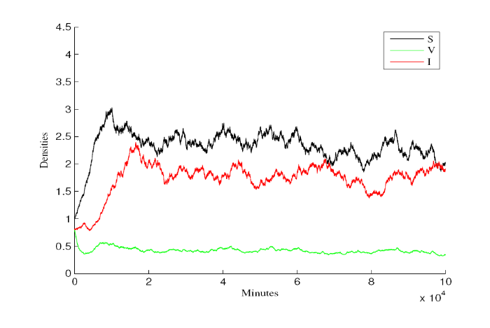
图2
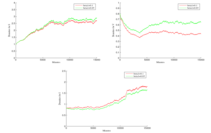
图3
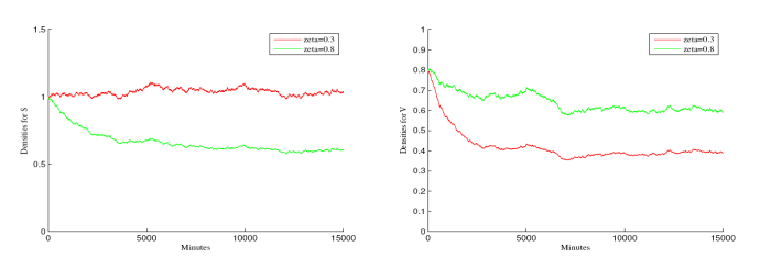
图4

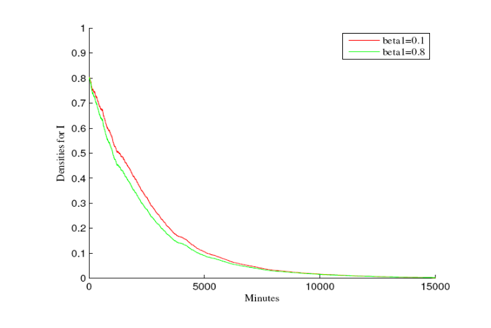
例 5.2 疾病的灭绝性在此例子中讨论, 设模型(1.2)初值S(0)=1, V(0)=0.8, I(0)=0.8, 以及其他参数取值为 \gamma=0.65, K=1.25, \beta=0.9, \beta_{1}=0.1, \tau=0.65, \delta=0.35, \zeta=0.3, \theta=0.2, \rho=0.8, \mu=0.5, \sigma_{1}=0.05, \sigma_{2}=0.05, \sigma_{3}=0.05, a=0.85, b=0.3. 这些参数值满足定理4.1的条件 R_{0}^{e}\approx0.9628<1,\ 0.5=\mu>0.5(\sigma_{1}^{2}\vee\sigma_{2}^{2}\vee\sigma_{3}^{2})=0.0012.
图5

图6
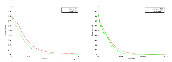
图7
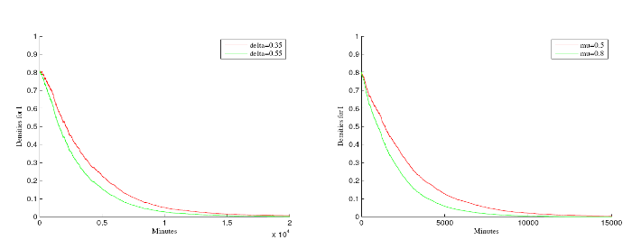
图8
参考文献
Traveling waves of a differential-difference diffusive Kermack-McKendrick epidemic model with age-structured protection phase
DOI:10.1016/j.jmaa.2021.125464 URL [本文引用: 1]
Dynamical behavior of a stochastic SEI epidemic model with saturation incidence and logistic growth
DOI:10.1016/j.physa.2019.04.228 URL [本文引用: 1]
A generalization of the Kermack-McKendrick deterministic epidemic model
DOI:10.1016/0025-5564(78)90006-8 URL [本文引用: 1]
A stochastic SIRI epidemic model with relapse and media coverage
Persistence and distribution of a stochastic susceptible-infected-removed epidemic model with varying population size
DOI:10.1016/j.physa.2017.04.114 URL [本文引用: 4]
Study on a susceptible-exposed-infected-recovered model with nonlinear incidence rate
The impact of media on the control of infectious diseases
DOI:10.1007/s10884-007-9075-0
PMID:32214759
[本文引用: 2]

We develop a three dimensional compartmental model to investigate the impact of media coverage to the spread and control of infectious diseases (such as SARS) in a given region/area. Stability analysis of the model shows that the disease-free equilibrium is globally-asymptotically stable if a certain threshold quantity, the basic reproduction number (), is less than unity. On the other hand, if, it is shown that a unique endemic equilibrium appears and a Hopf bifurcation can occur which causes oscillatory phenomena. The model may have up to three positive equilibria. Numerical simulations suggest that when and the media impact is stronger enough, the model exhibits multiple positive equilibria which poses challenge to the prediction and control of the outbreaks of infectious diseases.© Springer Science+Business Media, LLC 2007.
Analysis of the predator-prey interactions: A stochastic model incorporating disease invasion
The partially truncated Euler-Maruyama method and its stability and boundedness
Dynamic behavior of a stochastic SIRS epidemic model with media coverage
DOI:10.1002/mma.v41.14 URL [本文引用: 1]
Stationary distribution and probability density function of a stochastic SIRSI epidemic model with saturation incidence rate and logistic growth
DOI:10.1016/j.chaos.2020.110519 URL [本文引用: 1]
An algorithmic introduction to numerical simulation of stochastic differential equations
DOI:10.1137/S0036144500378302 URL [本文引用: 1]
Threshold dynamics of a stochastic SIHR epidemic model of COVID-19 with general population-size dependent contact rate
DOI:10.3934/mbe.2022195
PMID:35341295
[本文引用: 1]
In this paper, we propose a stochastic SIHR epidemic model of COVID-19. A basic reproduction number R_{0}^{s} is defined to determine the extinction or persistence of the disease. If R_{0}^{s} < 1 , the disease will be extinct. If R_{0}^{s} > 1 , the disease will be strongly stochastically permanent. Based on realistic parameters of COVID-19, we numerically analyze the effect of key parameters such as transmission rate, confirmation rate and noise intensity on the dynamics of disease transmission and obtain sensitivity indices of some parameters on R_{0}^{s} by sensitivity analysis. It is found that: 1) The threshold level of deterministic model is overestimated in case of neglecting the effect of environmental noise; 2) The decrease of transmission rate and the increase of confirmed rate are beneficial to control the spread of COVID-19. Moreover, our sensitivity analysis indicates that the parameters \beta , \sigma and \delta have significantly effects on R_0^s .
The impact of hospital resources and environmental perturbations to the dynamics of SIRS model
DOI:10.1016/j.jfranklin.2021.01.015 URL [本文引用: 1]
Stability and bifurcation analysis of an SIR epidemic model with logistic growth and saturated treatment
DOI:10.1016/j.chaos.2017.03.047 URL [本文引用: 1]
The effect of constant and pulse vaccination on SIS epidemic models incorporating media coverage
DOI:10.1016/j.cnsns.2008.06.024 URL [本文引用: 1]
The persistence and extinction of a stochastic SIS epidemic model with Logistic growth
Dynamical behavior of a higher order stochastically perturbed SIRI epidemic model with relapse and media coverage
DOI:10.1016/j.chaos.2020.110013 URL [本文引用: 1]
Dynamics of a stochastic predator-prey model with stage structure for predator and Holling type II functional response
DOI:10.1007/s00332-018-9444-3 [本文引用: 1]
Dynamical behavior of a stochastic HBV infection model with logistic hepatocyte growth
Persistence and extinction for an age-structured stochastic SVIR epidemic model with generalized nonlinear incidence rate
DOI:10.1016/j.physa.2018.09.016 URL [本文引用: 4]
Positivity preserving truncated Euler-Maruyama method for stochastic Lotka-Volterra competition model
DOI:10.1016/j.cam.2021.113566 URL [本文引用: 1]
Optimal vaccination strategy for an SIRS model with imprecise parameters and Lèvy noise
DOI:10.1016/j.jfranklin.2019.03.043 URL [本文引用: 2]
Stochastic functional Kolmogorov equations, I: Persistence
DOI:10.1016/j.spa.2021.09.007 URL [本文引用: 1]
Stochastic functional Kolmogorov equations II: Extinction
DOI:10.1016/j.jde.2021.05.043 URL [本文引用: 1]
Long-term analysis of a stochastic SIRS model with general incidence rates
DOI:10.1137/19M1246973 URL [本文引用: 1]
Dynamic threshold probe of stochastic SIR model with saturated incidence rate and saturated treatment function
DOI:10.1016/j.physa.2019.122300 URL [本文引用: 1]
Ergodic stationary distribution and extinction of a stochastic SIRS epidemic model with logistic growth and nonlinear incidence
Analysis of an SVEIS epidemic model with partial temporary immunity and saturation incidence rate
DOI:10.1016/j.apm.2011.07.044 URL [本文引用: 2]
Effect of media-induced social distancing on disease transmission in a two patch setting
DOI:10.1016/j.mbs.2011.01.005
PMID:21296092
[本文引用: 1]
We formulate an SIS epidemic model on two patches. In each patch, media coverage about the cases present in the local population leads individuals to limit the number of contacts they have with others, inducing a reduction in the rate of transmission of the infection. A global qualitative analysis is carried out, showing that the typical threshold behavior holds, with solutions either tending to an equilibrium without disease, or the system being persistent and solutions converging to an endemic equilibrium. Numerical analysis is employed to gain insight in both the analytically tractable and intractable cases; these simulations indicate that media coverage can reduce the burden of the epidemic and shorten the duration of the disease outbreak.Copyright © 2011 Elsevier Inc. All rights reserved.
The impact of media coverage on the transmission dynamics of human influenza
Global dynamics for an age-structured epidemic model with media impact and incomplete vaccination
DOI:10.1016/j.nonrwa.2016.04.009 URL [本文引用: 1]
Stochastic permanence of an SIQS epidemic model with saturated incidence and independent random perturbations
DOI:10.1016/j.physa.2016.01.059 URL [本文引用: 2]
Psychological effect on single-species population models in a polluted environment
DOI:S0025-5564(17)30142-6
PMID:28583848
[本文引用: 2]
We formulate and investigate the psychological effect of single-species population models in a polluted environment in this paper. For the deterministic single-species population model, the conditions that guarantee the local extinction and persistence in the mean are derived firstly. We then show that, around the pollution-free equilibrium, the stochastic single-species population is weakly persistent in the mean, and is stochastically permanent under some conditions. As a consequence, some numerical simulations demonstrate the efficiency of the main results.Copyright © 2017 Elsevier Inc. All rights reserved.
Dynamical behaviors of a heroin population model with standard incidence rates between distinct patches
DOI:10.1016/j.jfranklin.2021.04.024 URL [本文引用: 1]
Survival analysis of a single-species population model with fluctuations and migrations between patches
DOI:10.1016/j.apm.2019.12.023 URL [本文引用: 2]
Stability and extinction of SEIR epidemic models with generalized nonlinear incidence
DOI:10.1016/j.matcom.2018.09.029 URL [本文引用: 3]
Ergodic stationary distribution of a stochastic SIRS epidemic model incorporating media coverage and saturated incidence rate
DOI:10.1016/j.physa.2018.09.124
[本文引用: 1]
This study investigates the disease dynamics of a SIRS epidemic model as affected by environment fluctuations and media coverage. A unique global positive solution for the epidemic model is obtained. The stochastic endemic dynamics of the system is discussed by constructing suitable Lyapunov functions, and the ergodic stationary distribution of the stochastic model is established based on the method of Khasminskii. The extinction of the epidemic disease is also analyzed. (C) 2018 Elsevier B.V.
Dynamics of stochastically perturbed SIS epidemic model with vaccination
The threshold of a stochastic SIS epidemic model with vaccination
The effect of media coverage on threshold dynamics for a stochastic SIS epidemic model
DOI:10.1016/j.physa.2018.08.113
PMID:32288106
[本文引用: 1]
Media coverage is one of the important measures for controlling infectious diseases, but the effect of media coverage on diseases spreading in a stochastic environment still needs to be further investigated. Here, we present a stochastic susceptible-infected-susceptible (SIS) epidemic model incorporating media coverage and environmental fluctuations. By using Feller's test and stochastic comparison principle, we establish the stochastic basic reproduction number, which completely determines whether the disease is persistent or not in the population. If, the disease will go to extinction; if, the disease will also go to extinction in probability, which has not been reported in the known literatures; and if, the disease will be stochastically persistent. In addition, the existence of the stationary distribution of the model and its ergodicity are obtained. Numerical simulations based on real examples support the theoretical results. The interesting findings are that (i) the environmental fluctuation may significantly affect the threshold dynamical behavior of the disease and the fluctuations in different size scale population, and (ii) the media coverage plays an important role in affecting the stationary distribution of disease under a low intensity noise environment.© 2018 Elsevier B.V. All rights reserved.
