

1 引言
Cahn-Hilliard 方程由 Cahn 和 Hilliard[2]在 1958 年研究热力学两相物质之间的相互扩散现象时提出. 本文考虑如下的 Cahn-Hilliard 方程
其中
作为描述相场模型的最基本方程之一, Cahn-Hilliard 方程具有重要的研究意义和应用价值, 如材料科学[11],图像分析[6]和相变[4]等领域. 国内外学 者对Cahn-Hilliard 方程提出许多有效的数值解法, 如Zhang 等[14]构造无条件 能量稳定的有限差分格式, 提出了一种自适应时间步进策略, 这种策略避免了在数值模拟中使用大时间步长时可能导致的精度损失. 叶[13]利用 Legendre 拟谱法对Cahn-Hilliard 方程进行数值求解, 证明了离散解的存在唯一性, 并给出了最佳误差估计. Feng等[5]提 出全离散有限元格式, 并建立先验误差估计, 文中给出的全离散格式是最优阶的. 文献[13]介绍了一种求解 Cahn-Hilliard 方程的间断有限元方法, 这种方法在不诉诸任何迭代的情况下进行有效地求解, 并在效率、准确性和保持所需解的属性方面具有良好性能. 文献[8]利用间断有限体积元方法求解耦合 Navier-Stokes-Cahn-Hilliard 模型, 并对其质量守恒和能量耗散特性进行了分析, 该数值方法高效且易于处理具有不同类型边界条件的复杂几何形状. 在对 Cahn-Hilliard 方程进行数值模拟时, 间断有限体积元方法相较于其他方法,具有空间结构简单, 在时间相关问题中使用块对角质量矩阵等优点, 同时使用到的低阶元, 更适用于做网格灵活的自适应算法, 时间步长根据能量的演变而变化, 这样更好的解决了分割元素的自由度过大导致的计算量问题. 为了方法具有更好的稳定性, 时间离散选择全隐格式.
本文结构如下:第2节介绍 Cahn-Hilliard 方程间断有限体积元空间离散格式; 第3节结合全隐格式进行时间离散得到全离散格式, 并严格证明了质量守恒性质和离散能量耗散定律; 第5节通过数值算例验证所给格式的可行性和有效性. 最后, 第6节给出了结论.
2 间断有限体积元法
在区域
图1
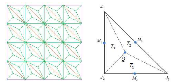
定义与相场变量
定义与化学势变量
式中,
设
如果
令
其中
引理 2.1 对于
对于
算子
定义分析中使用的
定义
将(1.1)式第一个式子两端同时乘上
设
在方程中
通过使用(2.6)式并结合
那么(1.1)式的弱格式为对
结合(2.3)-(2.10)式, Cahn-Hilliard 方程间断有限体积元方法的空间离散格式为: 对
其中
对于
假设
3 全离散格式
接下来, 我们再结合后向欧拉格式进行时间离散, 得到全离散格式. 令
初始条件为
定理 3.1
如果
接下来将证明时间离散质量守恒.
定理 3.2 令
证 令(3.1)式中的
这样就完成了定理的证明.证毕.
下面, 将验证 Cahn-Hilliard 系统的能量耗散性质. 首先定义相应的离散能量泛函
定理 3.3 令
证 令(3.1)式中的
对于双线性形式
同理令(3.1)式中的
为了更好的分析, 这里定义辅助双线性形式
通过定理3.1得到
(3.13)式的第一项计算可得
利用代数恒等式
根据
对
因此, 方程(3.13)左侧的第二项可写成以下形式
可以直接得到
最后, 将(3.1)-(3.21)式整理得到
这样我们就证明得出(3.1)式是无条件能量稳定的.证毕.
4 误差估计
引理 4.1(强制性) 存在一个与
引理 4.2(有界性) 对于
引理 4.3假设
那么存在一个独立于
上述引理使用文献[12] 中的方法可以得到. 方程(4.3)的一阶
我们引入一个椭圆投影算子
那么通过引理4.3我们有
注 4.1 上述引理对
定理 4.1 令
证 令
令
通过(4.6)式可将简化为
我们通过 Young-不等式得到
对于
可以将
其中
通过(4.13)式同理可得
将(4.12)-(4.15)式整理得到
根据引理4.3得到
最后通过三角不等式完成证明.
注 4.2 Cahn-Hilliard 方程全离散间断有限体积元方法的误差估计类似于定理 4.1 的证明.
注 4.3 其中
5 数值算例
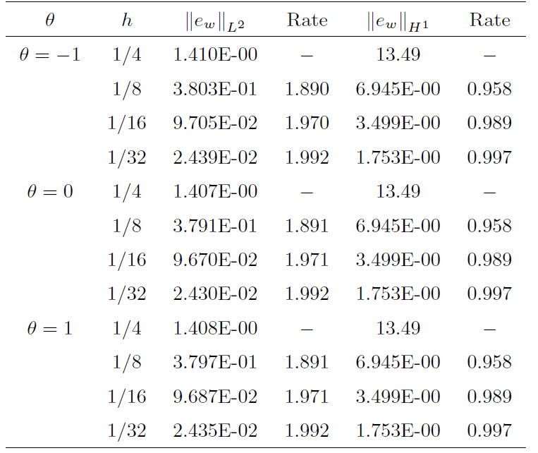
本节中, 我们将通过数值算例来验证所得数值格式的有效性. 算例 1, 我们使用一致网格剖分来验证
算例1 我们给出了所提出方法的数值误差和收敛速度. 选择 Cahn-Hilliard 方程的精确解为
定义误差

算例 2 在
图2
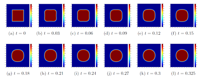
图3

图4
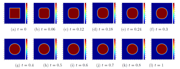
图5
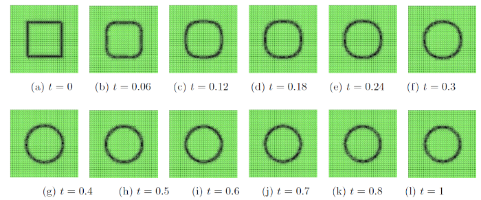
图6

图7
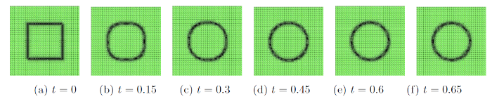
图8
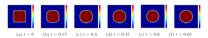
图9
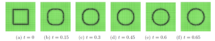
图10
6 总结
本文对 Cahn-Hilliard 方程的间断有限体积元方法进行了研究.空间离散利用间断有限体积元方法, 时间离散采用向后欧拉方法, 得到 Cahn-Hilliard 方程全离散格式, 验证了该格式质量守恒性质和离散能量耗散.最后通过数值实验提出了一种自适应时间步进策略计数数值格式的误差和收敛阶, 证明了该格式的有效性.
参考文献
A discontinuous finite volume element method for second-order elliptic problems
DOI:10.1002/num.v28.2 URL [本文引用: 1]
Free energy of a nonuniform system I: Interfacial free energy
DOI:10.1063/1.1744102
URL
[本文引用: 1]

It is shown that the free energy of a volume V of an isotropic system of nonuniform composition or density is given by : NV∫V [f0(c)+κ(▿c)2]dV, where NV is the number of molecules per unit volume, ▿c the composition or density gradient, f0 the free energy per molecule of a homogeneous system, and κ a parameter which, in general, may be dependent on c and temperature, but for a regular solution is a constant which can be evaluated. This expression is used to determine the properties of a flat interface between two coexisting phases. In particular, we find that the thickness of the interface increases with increasing temperature and becomes infinite at the critical temperature Tc, and that at a temperature T just below Tc the interfacial free energy σ is proportional to (Tc−T)32.
Unified analysis of finite volume methods for second order elliptic problems
DOI:10.1137/050643994 URL [本文引用: 1]
Fully discrete dynamic mesh discontinuous Galerkin methods for the Cahn-Hilliard equation of phase transition
DOI:10.1090/S0025-5718-07-01985-0 URL [本文引用: 1]
Analysis of a fully discrete finite element method for the phase field model and approximation of its sharp interface limits
DOI:10.1090/mcom/2004-73-246 URL [本文引用: 1]
Discovering phase field models from image data with the pseudo-spectral physics informed neural networks
DOI:10.1007/s42967-020-00105-2 [本文引用: 1]
Equal order discontinuous finite volume element methods for the Stokes problem
DOI:10.1007/s10915-015-9993-7 URL [本文引用: 1]
Discontinuous finite volume element method for a coupled Navier-Stokes-Cahn-Hilliard phase field model
DOI:10.1007/s10444-020-09758-2 [本文引用: 1]
Unconditionally energy stable discontinuous Galerkin schemes for the Cahn-Hilliard equation
DOI:10.1016/j.cam.2020.113375 URL
Numerical approximations of Allen-Cahn and Cahn-Hilliard equations
DOI:10.3934/dcds.2010.28.1669 URL [本文引用: 1]
Efficient energy stable numerical schemes for a phase field moving contact line model
DOI:10.1016/j.jcp.2014.12.046 URL [本文引用: 1]
A new discontinuous finite volume method for elliptic problems
DOI:10.1137/S0036142902417042 URL [本文引用: 3]
Cahn-Hilliard 方程的拟谱逼近
Legendre collocation approximation for Cahn-Hilliard equation
An adaptive time-stepping strategy for the Cahn-Hilliard equation
DOI:10.4208/cicp.300810.140411s
URL
[本文引用: 1]
This paper studies the numerical simulations for the Cahn-Hilliard equation which describes a phase separation phenomenon. The numerical simulation of the Cahn-Hilliard model needs very long time to reach the steady state, and therefore large time-stepping methods become useful. The main objective of this work is to construct the unconditionally energy stable finite difference scheme so that the large time steps can be used in the numerical simulations. The equation is discretized by the central difference scheme in space and fully implicit second-order scheme in time. The proposed scheme is proved to be unconditionally energy stable and mass-conservative. An error estimate for the numerical solution is also obtained with second order in both space and time. By using this energy stable scheme, an adaptive time-stepping strategy is proposed, which selects time steps adaptively based on the variation of the free energy against time. The numerical experiments are presented to demonstrate the effectiveness of the adaptive time-stepping approach.
