

1 引言与问题
尽管目前 HIV/AIDS预防和治疗取得了巨大进展, 但仍有一些低收入和中等收入国家受到 HIV 流行的影响. 据估计, 截止到2020 年底全球有 3760 万 HIV 感染者, 大约 680,000 人死于与AIDS相关的疾病, 其中大多数在东部和南部非洲. 在影响 HIV/AIDS 传播和分布的所有因素中, 人群的扩散被认为是一个重要因素. 这促使关于HIV/AIDS 空间传播动力学的研究工作广泛展开. 例如, Cuadros 等[2] 利用一种基于空间变量的模型在几个非洲国家创建高分辨率的艾滋病毒感染率估计图. Ayalew 等[3] 比较了三种空间 HIV 模型, 以估计南非不同地区的艾滋病毒感染率. Wu 和 Zhao[4] 研究了一类带有抗逆转录病毒治疗的年龄结构空间艾滋病毒流行病模型的动力学行为. Zhao 等[5] 建立了一类具有三年龄段的 HIV/AIDS 流行病模型, 并进行了动力学和最优控制分析. 其他一些时空结构 HIV 感染模型也已被用来研究 HIV 在宿主体内的传播动力学(参见文献[6⇓⇓⇓-10]).
事实上, 随着时间的推移, HIV 感染者可能会发展成艾滋病或保持在无症状阶段, 这在很大程度上取决于感染者的感染年龄, 即个体感染 HIV 后的时间. 因此有必要将感染年龄纳入空间 HIV/AIDS 模型, 以揭示该疾病传播的动力学机制, 这就是所谓的“年龄-空间结构”. 除了文献[4-5]所做的研究工作之外, 年龄-空间结构也被一些学者在建立其他传染病模型时所考虑. 最近, Chekroun和Kuniya[11]研究了具有 Neumann 边界条件的年龄空间结构SIR 流行病模型的全局动力学. Yang等[12]研究了年龄结构空间布鲁氏菌病模型的阈值动力学行为. Liu 等[13]研究了具有年龄结构和空间扩散的多群体SEIR流行病模型的全局演化行为. Wang等[14]建立了一类具有年龄-空间结构的 HIV 感染模型并研究了模型解的全局动力学行为. 值得提出的是, 上述这些模型都是考虑了齐次 Neumann 边界条件. 然而, 当空间区域的边界具有对个体生存不利的环境 (例如, 沼泽、沙漠或高山) 时, 模型更适合考虑齐次狄利克雷边界条件 (参见文献[15-16]). 有鉴于此, 具有狄利克雷边界条件的空间模型已被用于研究相关传染病的动力学传播. 例如, Chekroun 和 Kuniya[17]分析了 Dirichlet 边界条件下具有年龄-空间结构 SIR 反应扩散传染病模型的阈值动力学. Wang等[18]在齐次 Dirichlet 边界条件下分析了年龄-空间结构口蹄疫模型的时空动力学.
受到上述研究工作的启发, 为了研究人群扩散、感染年龄和 Dirichlet 边界条件环境对人群中 HIV/AIDS 传播的综合影响, 本文建立如下模型
模型的初值条件和齐次 Dirichlet 边界条件如下所示
其中,
令
由于
其中
接下来, 我们致力于研究系统 (1.5) 的动力学行为.
2 系统(1.5)的适定性
为了研究系统 (1.5) 的适定性,我们首先做出如下假设.
(1) 模型参数
(2)
(3)
我们令空间
根据格林函数
进一步地, 我们可得系统(1.5)解的全局存在性和一致有界性的结论.
其中
由此, 我们可知当(2.1)式存在解
令
注意到
对任意固定的
定义
以及
令
这意味着
假设
于是利用 Gronwall 不等式, 可得
3 模型的基本再生数
此节中, 我们致力于推导出系统 (1.5) 的基本再生数泛函表达式. 根据命题 4.1 和引理 4.1[17], 可知方程
有唯一的非负解
根据文献[25], 我们定义再生算子
4 模型无病平衡态的全局吸引性
此节中, 我们讨论系统 (1.5) 无病平衡态
其中
假设存在
引理证毕.
这意味着
继而可得
其中
5 疾病的一致持久性
此节中, 我们证明当
选取
我们用
因此, 对于
继而可知
其中
这里
从而可得
设
这与
设
对
由于
接下来, 我们证明系统 (1.5) 存在空间依赖的正稳态
然后,正稳态满足方程
从而可得
其中 Itô是关于
以及从
其中
其中
一方面, 由于
6 数值模拟
在本节中, 我们根据中国50岁及以上感染艾滋病人群的报告病例, 对系统 (1.5) 进行数值模拟. 与文献[17]类似, 我们考虑矩形域
其中
利用文献[27,3.1.2 节]中的 Fredholm 离散化方法, 我们可以得到
图 1
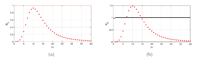
图 1
(a)
图 2
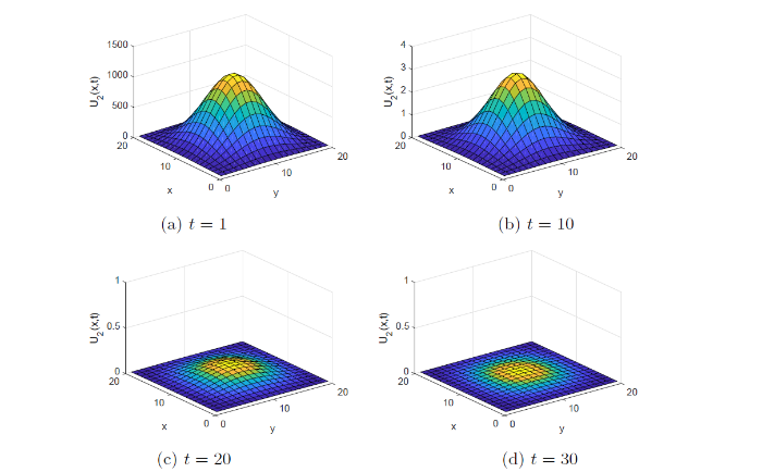
图 3
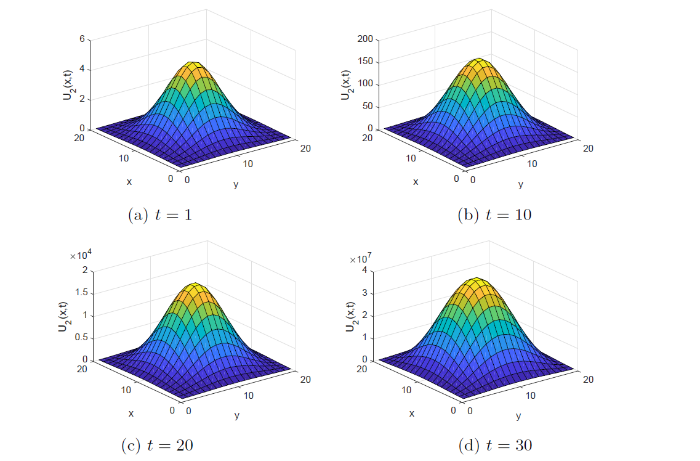
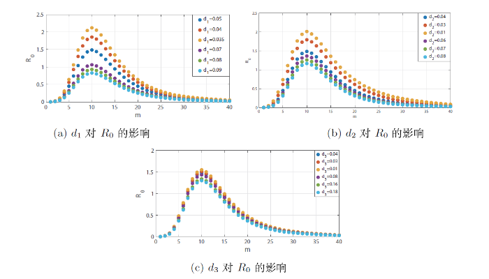
图 4
7 结论
在本文中, 我们建立了一类具有齐次 Dirichlet 边界条件的年龄空间结构 HIV/AIDS 传染病模型. 这种边界条件给动力学分析带来了挑战. 首先, 由于系统的无病稳态是非常数的, 即使模型参数是空间无关的, 这与齐次Neumann 边界条件下的空间同质模型的结论不同. 其次, 由于反应扩散方程和积分方程的耦合系统的耗散性不能直接得到, 我们证明了系统的一致持久性之后, 不能直接获得依赖于空间的正稳态解的存在性. 为了克服这些困难, 我们首先研究了系统的适定性, 并导出了基本再生数
参考文献
Mapping the spatial variability of HIV infection in Sub-Saharan Africa: Efective information for localized HIV prevention and control
DOI:10.1038/s41598-017-09464-y
PMID:28831171
[本文引用: 1]

Under the premise that in a resource-constrained environment such as Sub-Saharan Africa it is not possible to do everything, to everyone, everywhere, detailed geographical knowledge about the HIV epidemic becomes essential to tailor programmatic responses to specific local needs. However, the design and evaluation of national HIV programs often rely on aggregated national level data. Against this background, here we proposed a model to produce high-resolution maps of intranational estimates of HIV prevalence in Kenya, Malawi, Mozambique and Tanzania based on spatial variables. The HIV prevalence maps generated highlight the stark spatial disparities in the epidemic within a country, and localize areas where both the burden and drivers of the HIV epidemic are concentrated. Under an era focused on optimal allocation of evidence-based interventions for populations at greatest risk in areas of greatest HIV burden, as proposed by the Joint United Nations Programme on HIV/AIDS (UNAIDS) and the United States President's Emergency Plan for AIDS Relief (PEPFAR), such maps provide essential information that strategically targets geographic areas and populations where resources can achieve the greatest impact.
A comparison of Bayesian spatial models for HIV mapping in South Africa
DOI:10.3390/ijerph182111215
URL
[本文引用: 1]
Despite making significant progress in tackling its HIV epidemic, South Africa, with 7.7 million people living with HIV, still has the biggest HIV epidemic in the world. The Government, in collaboration with developmental partners and agencies, has been strengthening its responses to the HIV epidemic to better target the delivery of HIV care, treatment strategies and prevention services. Population-based household HIV surveys have, over time, contributed to the country’s efforts in monitoring and understanding the magnitude and heterogeneity of the HIV epidemic. Local-level monitoring of progress made against HIV and AIDS is increasingly needed for decision making. Previous studies have provided evidence of substantial subnational variation in the HIV epidemic. Using HIV prevalence data from the 2016 South African Demographic and Health Survey, we compare three spatial smoothing models, namely, the intrinsically conditionally autoregressive normal, Laplace and skew-t (ICAR-normal, ICAR-Laplace and ICAR-skew-t) in the estimation of the HIV prevalence across 52 districts in South Africa. The parameters of the resulting models are estimated using Bayesian approaches. The skewness parameter for the ICAR-skew-t model was not statistically significant, suggesting the absence of skewness in the HIV prevalence data. Based on the deviance information criterion (DIC) model selection, the ICAR-normal and ICAR-Laplace had DIC values of 291.3 and 315, respectively, which were lower than that of the ICAR-skewed t (348.1). However, based on the model adequacy criterion using the conditional predictive ordinates (CPO), the ICAR-skew-t distribution had the lowest CPO value. Thus, the ICAR-skew-t was the best spatial smoothing model for the estimation of HIV prevalence in our study.
Mathematical analysis of an age-structured HIV/AIDS epidemic model with HAART and spatial diffusion
DOI:10.1016/j.nonrwa.2021.103289 URL [本文引用: 2]
Dynamic analysis and optimal control three-age-class HIV/AIDS epidemic model in China
Dynamical analysis of a nonlocal delayed and diffusive HIV latent infection model with spatial heterogeneity
DOI:10.1016/j.jfranklin.2021.05.014 URL [本文引用: 2]
Threshold dynamics of a delayed nonlocal reaction-diffusion HIV infection model with both cell-free and cell-to-cell transmissions
DOI:10.1016/j.jmaa.2020.124047 URL [本文引用: 1]
A delayed reaction-diffusion viral infection model with nonlinear incidences and cell-to-cell transmission
DOI:10.1142/S179352452150100X
URL
[本文引用: 1]
In this paper, we propose a reaction–diffusion viral infection model with nonlinear incidences, cell-to-cell transmission, and a time delay. We impose the homogeneous Neumann boundary condition. For the case where the domain is bounded, we first study the well-posedness. Then we analyze the local stability of homogeneous steady states. We establish a threshold dynamics which is completely characterized by the basic reproduction number. For the case where the domain is the whole Euclidean space, we consider the existence of traveling wave solutions by using the cross-iteration method and Schauder’s fixed point theorem. Finally, we study how the speed of spread in space affects the spread of cells and viruses. We obtain the existence of the wave speed, which is dependent on the diffusion coefficient.
Time periodic reaction-diffusion equations for modeling 2-LTR dynamics in HIV-infected patients
DOI:10.1016/j.nonrwa.2020.103184 URL [本文引用: 1]
具有时滞扩散效应的病原体-免疫模型的稳定性及分支
Stability and Bifurcation analysis of a delayed diffusive pathogen-immune model
An infection age-space structured SIR epidemic model with Neumann boundary condition
DOI:10.1080/00036811.2018.1551997 URL [本文引用: 6]
Threshold dynamics of an age-space structured brucellosis disease model with Neumann boundary condition
DOI:10.1016/j.nonrwa.2019.04.013 URL [本文引用: 3]
Global behavior of a multi-group SEIR epidemic model with age structure and spatial diffusion
DOI:10.3934/mbe.2020372
PMID:33378896
[本文引用: 1]
Different epidemic models with one or two characteristics of multi-group, age structure and spatial diffusion have been proposed, but few models take all three into consideration. In this paper, a novel multi-group SEIR epidemic model with both age structure and spatial diffusion is constructed for the first time ever to study the transmission dynamics of infectious diseases. We first analytically study the positivity, boundedness, existence and uniqueness of solution and the existence of compact global attractor of the associated solution semiflow. Based on some assumptions for parameters, we then show that the disease-free steady state is globally asymptotically stable by utilizing appropriate Lyapunov functionals and the LaSalle's invariance principle. By means of Perron-Frobenius theorem and graph-theoretical results, the existence and global stability of endemic steady state are ensured under appropriate conditions. Finally, feasibility of main theoretical results is showed with the aid of numerical examples for model with two groups which is important from the viewpoint of applications.
Global threshold dynamics of an infection age-space structured HIV infection model with Neumann boundary condition
Analysis of a spatial memory model with nonlocal maturation delay and hostile boundary condition
DOI:10.3934/dcds.2020249 URL [本文引用: 1]
On Dirichlet problem for a class of delayed reaction-diffusion equations with spatial non-locality
Global threshold dynamics of an infection age-structured SIR epidemic model with diffusion under the Dirichlet boundary condition
DOI:10.1016/j.jde.2020.04.046 URL [本文引用: 6]
Temporal-spatial analysis of an age-space structured foot-and-mouth disease model with Dirichlet boundary condition
DOI:10.1063/5.0048282 URL [本文引用: 1]
Global stability of an infection-age structured HIV-1 model linking within-host and between-host dynamics
DOI:10.1016/j.mbs.2015.02.003
PMID:25686694
[本文引用: 1]
Although much evidence shows the inseparable interaction between the within-host progression of HIV-1 infection and the transmission of the disease at the population level, few models coupling the within-host and between-host dynamics have been developed. In this paper, we adopt the nested approach, viewing the transmission rate at each stage (primary, chronic, and AIDS stage) of HIV-1 infection as a saturated function of the viral load, to formulate an infection-age structured epidemic model. We explicitly link the individual and the host population scale, and derive the basic reproduction number R0 for the coupled system. To analyze the model and perform a detailed global dynamics analysis, two Lyapunov functionals are constructed to prove the global asymptotical stability of the disease-free and endemic equilibria. Theoretical results indicate that R0 provides a threshold value determining whether or not the disease dies out. Numerical simulations are presented to quantitatively investigate the influence of the within-host viral dynamics on between-host transmission dynamics. The results suggest that increasing the effectiveness of inhibitors can decrease the basic reproduction number, but can also increase the overall infected population because of a lower disease-induced mortality rate and a longer lifespan of HIV infected individuals. Copyright © 2015 Elsevier Inc. All rights reserved.
Threshold dynamics of a delayed nonlocal reaction-diffusion HIV infection model with both cell-free and cell-to-cell transmissions
DOI:10.1016/j.jmaa.2020.124047 URL [本文引用: 1]
Threshold dynamics of an age-space structured SIR model on heterogeneous environment
DOI:10.1016/j.aml.2019.03.009 URL [本文引用: 1]
On the Dirichlet problem for elliptic systems
DOI:10.1080/00036818608839592 URL [本文引用: 1]
Spatial invasion threshold of Lyme disease
Monotone Dynamical Systems: An Introduction to the Theory of Competitive and Cooperative Systems
The spectral approximation of linear operators with applications to the computation of eigenelements of differential and integral operators
DOI:10.1137/1023099 URL [本文引用: 1]
