西藏自治区包虫病传播的数学建模及动力学分析

图1 包虫病在人、犬、家畜中的传播示意图

$\begin{matrix} \left\{ \begin{array}{ll}\displaystyle \frac{{\rm d}H_{s}}{{\rm d}t}=A_{h}+\mu_{2}H_{i}+\mu_{1}qH_{e}-(1-p)\beta_{1}D_{i}H_{s}-d_{h}H_{s},\\ [3mm]\displaystyle \frac{{\rm d}H_{e}}{{\rm d}t}=(1-p)\beta_{1}D_{i}H_{s}-\mu_{1}qH_{e}-d_{h}H_{e}-(1-q)\omega H_{e}, \\[3mm]\displaystyle \frac{{\rm d}H_{i}}{{\rm d}t}=(1-q)\omega H_{e}-\mu_{2}H_{i}-d_{h}H_{i}, \\[3mm]\displaystyle \frac{{\rm d}D_{s}}{{\rm d}t}=b_{d}N_{d}-(1-p)\beta_{2}\varepsilon L_{i}D_{s}-(d+\theta)D_{s}-(b_{d}-d)\frac{N_{d}}{K}D_{s}, \\[3mm]\displaystyle \frac{{\rm d}D_{i}}{{\rm d}t}=(1-p)\beta_{2}\varepsilon L_{i}D_{s}-(d+\theta)D_{i}-(b_{d}-d)\frac{N_{d}}{K}D_{i}, \\[3mm] \displaystyle \frac{{\rm d}L_{s}}{{\rm d}t}=(d_{l}+\varepsilon)M-(1-p)\beta_{3}D_{i}L_{s}-(d_{l}+\varepsilon)L_{s}, \\[3mm]\displaystyle \frac{{\rm d}L_{i}}{{\rm d}t}=(1-p)\beta_{3}D_{i}L_{s}-(d_{l}+\varepsilon)L_{i}. \end{array} \right.\end{matrix}$

(2.1)

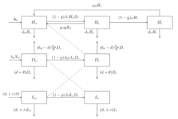
模型中的参数均为正值, 其中 $A_{h}$ 表示人口每年新增数量; $d_{h}, d_{l}$ 分别表示人, 家畜的自然死亡率; $\beta_{1}, \beta_{2}, \beta_{3}$ 分别表示人, 犬, 家畜的感染系数; $\frac{1}{\omega}$ 表示潜伏期人群转化成发病人群的平均潜伏时间; $\mu_{1}, \mu_{2}$ 分别表示潜伏人群和发病人群的治愈率系数; $q$ 表示潜伏人群接受治疗的比例; $p$ 表示地区宣传教育的影响系数; $\varepsilon$ 表示家畜的屠宰比例.

根据问题的实际含义我们仅在区域

$\Gamma=\{(H_{s},H_{e},H_{i},D_{s},D_{i},L_{s},L_{i})| H_{s}\geq0, H_{e}\geq0, H_{i}\geq0, D_{s}\geq0, D_{i}\geq0, L_{s}\geq0, L_{i}\geq0$

$H_{s}+H_{e}+H_{i}\leq\frac{A_{h}}{d_{h}}, D_{s}+D_{i}\leq\frac{K(b_{d}-d-\theta)}{b_{d}-d}, L_{s}+L_{i}=M\}$

中讨论系统 (2.1) 解的性态. 并且容易验证 $\Gamma$ 是系统 (2.1) 的正向不变域.

显然, 系统 (2.1) 总存在一个平凡平衡点 $E_{*}$ 和一个无病平衡点 $E_{0}$

$E_{*}=(\frac{A_{h}}{d_{h}},0,0,0,0,M,0), E_{0}=(\frac{A_{h}}{d_{h}},0,0,\frac{K(b_{d}-d-\theta)}{b_{d}-d},0,M,0).$

利用下一代矩阵的方法^[16], 令 $F$ 和 $V$ 分别表示新增感染项和保留转移项, 则基本再生数 $R_{0}$ 可由 $\rho(FV^{\dashv})$ 计算得出

$R_{0}=\sqrt[2]{\frac{(1-p)\beta_{3}M}{b_{d}}\cdot\frac{(1-p)\varepsilon\beta_{2}K(b_{d}-d-\theta)}{(d_{l}+\varepsilon)(b_{d}-d)}}.$

进一步, 当 $R_{0}>1$ 时系统 $(2.1)$ 存在唯一的地方病平衡点 $E^{*}=(H_{s}^{*},H_{e}^{*},H_{i}^{*},D_{s}^{*},D_{i}^{*},L_{s}^{*},L_{i}^{*})$ , 其中

$H_{s}^{*}=\frac{\mu_{1}q+d_{h}+(1-q)\omega}{(1-p)\beta_{1}D_{i}^{*}}H_{e}^{*},$

$H_{e}^{*}=\frac{A_{h}(\mu_{2}+d_{h})(1-p)\beta_{1}D_{i}^{*}}{d_{h}[(1-q)\omega(1-p)\beta_{1}D_{i}^{*}+(\mu_{2}+d_{h})(\mu_{1}q+d_{h}+(1-q)\omega)+(\mu_{2}+d_{h})(1-p)\beta_{1}D_{i}^{*}]},$

$H_{i}^{*}=\frac{(1-q)\omega}{\mu_{2}+d_{h}}H_{e}^{*}, D_{s}^{*}=\frac{K(b_{d}-d-\theta)}{b_{d}-d}-D_{i}^{*}, D_{i}^{*}=\frac{(d_{l}+\varepsilon)L_{i}^{*}}{\beta_{3}(1-p)(M-L_{i}^{*})}, L_{s}^{*}=M-L_{i}^{*},$

$L_{i}^{*}=\frac{b_{d}(d_{l}+\varepsilon)(b_{d}-d)(R_{0}^{2}-1)}{(1-p)^{2}\beta_{2}\beta_{3}\varepsilon K(b_{d}-d-\theta)+(1-p)\beta_{2}\varepsilon(d_{l}+\varepsilon)(b_{d}-d)}.$

3 平衡点的稳定性

定理3.1 平凡平衡点 $E_{*}$ 总是不稳定的.

证系统 (2.1) 在 $E_{*}$ 处线性化系统的特征方程为

$(\lambda+d_{h})(\lambda+d_{l}+\varepsilon)^{2}(\lambda+d+\theta)(\lambda+\mu_{2}+d_{h})(\lambda+\mu_{1}q+d_{h}+(1-q)\omega)(\lambda-(b_{d}-d-\theta))=0.$

而 $\lambda=b_{d}-d-\theta>0$ 是其正特征根, 所以 $E_{*}$ 总是不稳定的. 证毕.

定理3.2 当 $R_{0}<1$ 时, 无病平衡点 $E_{0}=(\frac{A_{h}}{d_{h}},0,0,\frac{K(b_{d}-d-\theta)}{b_{d}-d},0,M,0)$ 全局渐近稳定;当 $R_{0}>1$ 时, $E_{0}$ 不稳定.

证系统 (2.1) 在 $E_{0}$ 处线性化系统的特征方程为

$\begin{matrix}&& (\lambda+d_{h})(\lambda+\mu_{2}+d_{h})(\lambda+\mu_{1}q+d_{h}+(1-q)\omega)(\lambda+(b_{d}-d-\theta)) (\lambda+d_{l}+\varepsilon)\\ &&\cdot [\lambda^{2}+(d_{l}+b_{d}+\varepsilon)\lambda+b_{d}(d_{l}+\varepsilon)(1-R^{2}_{0})]=0.\end{matrix}$

显然, 该特征方程有五个实根且都小于零, 另外两个根为

$\lambda=\frac{-(d_{l}+b_{d}+\varepsilon)}{2}\pm\frac{\sqrt{(d_{l}+b_{d}+\varepsilon)^{2}-4b_{d}(d_{l}+\varepsilon)(1-R^{2}_{0})}}{2}.$

所以当 $R_{0}<1$ 时, $E_{0}$ 是局部渐近稳定; 而当 $R_{0}>1$ 时, $E_{0}$ 不稳定.

下面证明当 $R_{0}<1$ 时, $E_{0}$ 全局渐近稳定. 因为系统 (2.1) 的前三个方程独立于其余方程, 所以可将系统 (2.1) 分为两个子系统进行研究. 首先考虑后四个方程所构成的子系统

$\begin{matrix} \left\{ \begin{array}{l} \frac{{\rm d}D_{s}}{{\rm d}t}=b_{d}N_{d}-(1-p)\beta_{2}\varepsilon L_{i}D_{s}-(d+\theta)D_{s}-(b_{d}-d)\frac{N_{d}}{K}D_{s}, \\[3mm] \frac{{\rm d}D_{i}}{{\rm d}t}=(1-p)\beta_{2}\varepsilon L_{i}D_{s}-(d+\theta)D_{i}-(b_{d}-d)\frac{N_{d}}{K}D_{i}, \\[3mm] \frac{{\rm d}L_{s}}{{\rm d}t}=(d_{l}+\varepsilon)M-(1-p)\beta_{3}D_{i}L_{s}-(d_{l}+\varepsilon)L_{s}, \\[3mm] \frac{{\rm d}L_{i}}{{\rm d}t}=(1-p)\beta_{3}D_{i}L_{s}-(d_{l}+\varepsilon)L_{i}. \end{array} \right.\end{matrix}$

(3.1)

由于 $\lim\limits_{ t\rightarrow \infty}N_{d}(t)=\frac{K(b_{d}-d-\theta)}{b_{d}-d}$ , 所以将 $N_{d}(t)=\frac{K(b_{d}-d-\theta)}{b_{d}-d}$ 带入, 可得系统 (3.1) 的极限系统

$\begin{matrix} \left\{ \begin{array}{l} \frac{{\rm d}D_{i}}{{\rm d}t}=(1-p)\beta_{2}\varepsilon L_{i}(\frac{K(b_{d}-d-\theta)}{b_{d}-d}-D_{i})-b_{d}D_{i}, \\[3mm] \frac{{\rm d}L_{i}}{{\rm d}t}=(1-p)\beta_{3}D_{i}(M-L_{i})-(d_{l}+\varepsilon)L_{i}. \end{array} \right.\end{matrix}$

(3.2)

由极限系统的理论可知, 系统 (3.1) 平衡点的稳定性等价于系统 (3.2) 平衡点的稳定性. 所以现在问题转化为讨论系统 (3.2) 的平衡点 (0,0) 的全局稳定性.

设 $(D_{i}(t),L_{i}(t))$ 为系统(3.2)在 $\Gamma$ 中的任意解, 定义 Lyapunov 函数为

$V(D_{i},L_{i})=\frac{(1-p)\beta_{3}M}{b_{d}}D_{i}+L_{i}.$

将函数 $V$ 沿系统 (3.2) 求导可得

$\begin{matrix}\frac{{\rm d}V}{{\rm d}t}&=&\frac{(1-p)\beta_{3}M}{b_{d}}((1-p)\beta_{2}\varepsilon L_{i}(\frac{K(b_{d}-d-\theta)}{b_{d}-d}-D_{i})-b_{d}D_{i})\\&&+(1-p)\beta_{3}D_{i}(M-L_{i})-(d_{l}+\varepsilon)L_{i}\\&\leq&\frac{(1-p)^{2}\beta_{2}\beta_{3}\varepsilon MK(b_{d}-d-\theta)}{b_{d}(b_{d}-d)}L_{i}-(d_{l}+\varepsilon)L_{i}\\&=&(R^{2}_{0}-1)(d_{l}+\varepsilon)L_{i}.\end{matrix}$

则当 $R_{0}<1$ 时 $\frac{{\rm d}V}{{\rm d}t}\leq0,$ 并且 $\frac{{\rm d}V}{{\rm d}t}=0$ 当且仅当 $L_{i}=0.$ 即

$E=\{(D_{i},L_{i})|\frac{{\rm d}V}{{\rm d}t}=0\}=\{(D_{i},0)\},$

而 $(0,0)$ 是系统 (3.2) 在 $E$ 中的唯一正向不变集, 由 LaSalle's 不变集原理可知 $(0,0)$ 是全局渐近稳定的.

接下来考虑系统 (2.1) 前三个方程所构成的子系统

$\begin{matrix} \left\{ \begin{array}{l} \frac{{\rm d}H_{s}}{{\rm d}t}=A_{h}+\mu_{2}H_{i}+\mu_{1}qH_{e}-(1-p)\beta_{1}D_{i}H_{s}-d_{h}H_{s},\\ [3mm] \frac{{\rm d}H_{e}}{{\rm d}t}=(1-p)\beta_{1}D_{i}H_{s}-\mu_{1}qH_{e}-d_{h}H_{e}-(1-q)\omega H_{e}, \\[3mm] \frac{{\rm d}H_{i}}{{\rm d}t}=(1-q)\omega H_{e}-\mu_{2}H_{i}-d_{h}H_{i}. \end{array} \right.\end{matrix}$

(3.3)

当 $t\rightarrow\infty$ 时 $D_{i}\rightarrow0$ . 计算可得, 当 $t\rightarrow\infty$ 时 $H_{e}\rightarrow0, H_{i}\rightarrow0, H_{s}\rightarrow \frac{A_{h}}{d_{h}}.$ 故系统 (3.3) 的平衡点 $(\frac{A_{h}}{d_{h}},0,0)$ 是全局渐近稳定的.

综上所述, 当 $R_{0}<1$ 时, 系统 (2.1) 的无病平衡点 $E_{0}$ 是全局渐近稳定的.证毕.

定理3.3 当 $R_{0}>1$ 时, 地方病平衡点 $E^{*}=(H_{s}^{*},H_{e}^{*},H_{i}^{*},D_{s}^{*},D_{i}^{*},L_{s}^{*},L_{i}^{*})$ 全局渐进稳定.

证类似于上面的证明方法, 先考虑极限系统 (3.2) 的平衡点 $(D_{i}^{*},L_{i}^{*})$ . 设 Lyapunov 函数为

$L(D_{i},L_{i})=\omega_{1}(D_{i}-D^{*}_{i}-D^{*}_{i}\ln\frac{D_{i}}{D^{*}_{i}})+\omega_{2}(L_{i}-L^{*}_{i}-L^{*}_{i}\ln\frac{L_{i}}{L^{*}_{i}}).$

选取 $\omega_{1}>0,$ 且 $\omega_{1}, \omega_{2}$ 满足

$\omega_{1}\frac{(1-p)\beta_{2}\varepsilon }{D^{*}_{i}}(\frac{K(b_{d}-d-\theta)}{b_{d}-d}-D^{*}_{i})=\omega_{2}\frac{(1-p)\beta_{3}}{L^{*}_{i}}(M-L^{*}_{i}).$

显然, $L(D_{i},L_{i})$ 是正定无穷大函数, 将函数 $L$ 沿系统 (3.2) 求导可得

$\begin{matrix}\frac{{\rm d}L}{{\rm d}t}&=&\omega_{1}\frac{D_{i}-D^{*}_{i}}{D_{i}}\frac{{\rm d}D_{i}}{{\rm d}t}+\omega_{2}\frac{L_{i}-L^{*}_{i}}{L_{i}}\frac{{\rm d}L_{i}}{{\rm d}t}\\&=&\left(\begin{array}{cc}D_{i}-D^{*}_{i}~&L_{i}-L^{*}_{i}\end{array}\right)\\&&\cdot \left[\begin{array}{cc} -\omega_{1}\frac{(1-p)\beta_{2}\varepsilon K(b_{d}-d-\theta)}{D_{i}D^{*}_{i}(b_{d}-d)}L_{i}~& \omega_{1}\frac{(1-p)\beta_{2}\varepsilon }{D^{*}_{i}}(\frac{K(b_{d}-d-\theta)}{b_{d}-d}-D^{*}_{i})\\[3mm] \omega_{2}\frac{(1-p)\beta_{3}}{L^{*}_{i}}(M-L^{*}_{i})~& -\omega_{2}\frac{(1-p)\beta_{3}M}{L_{i}L^{*}_{i}}D_{i}\end{array}\right]\left(\begin{array}{cc}D_{i}-D^{*}_{i}\\L_{i}-L^{*}_{i}\end{array}\right)\\&\leq& 0.\end{matrix}$

且等号仅在 $D_{i}=D_{i}^{*}, L_{i}=L_{i}^{*}$ 处成立, 故系统 (3.2) 的平衡点 $(D_{i}^{*},L_{i}^{*})$ 全局渐近稳定.

接下来考虑子系统 (3.3). 当 $t\rightarrow\infty$ 时 $D_{i}\rightarrow D^{*}$ . 故子系统 (3.3) 的极限系统为

$\begin{matrix} \left\{ \begin{array}{l} \frac{{\rm d}H_{s}}{{\rm d}t}=A_{h}+\mu_{2}H_{i}+\mu_{1}qH_{e}-(1-p)\beta_{1}D^{*}_{i}H_{s}-d_{h}H_{s},\\[3mm] \frac{{\rm d}H_{e}}{{\rm d}t}=(1-p)\beta_{1}D^{*}_{i}H_{s}-\mu_{1}qH_{e}-d_{h}H_{e}-(1-q)\omega H_{e}, \\[3mm] \frac{{\rm d}H_{i}}{{\rm d}t}=(1-q)\omega H_{e}-\mu_{2}H_{i}-d_{h}H_{i}. \end{array} \right.\end{matrix}$

(3.4)

显然, 系统 (3.4) 为一个线性系统, 其特征方程为

$\lambda^{3}+a_{1}\lambda^{2}+a_{2}\lambda+a_{3}=0,$

其中

$\begin{matrix} a_{1}&=& \mu_{1}q+\mu_{2}+3d_{h}+(1-q)\omega+(1-p)\beta_{1}D_{i}^{*},\\ a_{2}&= &(\mu_{2}+d_{h})(\mu_{1}q+d_{h}+(1-q)\omega)+d_{h}\mu_{1}q+((1-p)\beta_{1}D_{i}^{*}+d_{h})(\mu_{2}+2d_{h}+(1-q)\omega), \\ a_{3}&=&d_{h}(1-p)\beta_{1}D_{i}^{*}(\mu_{2}+d_{h}+(1-q)\omega)+d_{h}(\mu_{2}+d_{h})(\mu_{1}q+d_{h}+(1-q)\omega). \end{matrix}$

由于 $a_{1}>0, a_{3}>0, a_{1}a_{2}-a_{3}>0,$ 故其特征根都具有负实部, 所以系统 (3.4) 的平衡点 $(H_{s}^{*},H_{e}^{*},H_{i}^{*})$ 全局渐近稳定.

综上所述, 当 $R_{0}<1$ 时, 系统 (2.1) 的地方病平衡点 $E^{*}$ 全局渐近稳定.证毕.

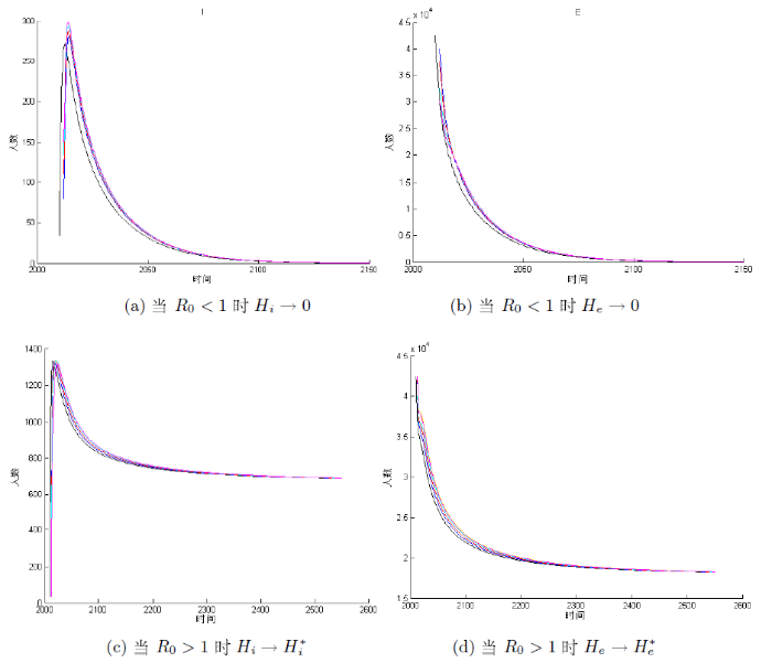
如图2 所示, 当取定参数, 使得 $R_{0}<1$ 时, 取不同初值, 潜伏期人数与发病人数最终都会趋于零, 疾病消失; 当 $R_{0}>1$ 时, 取不同的初值, 潜伏期人数与发病人数最终都会稳定于同一个平衡点, 形成地方疾病.

图2

图2 潜伏期人数与发病人数随时间变化图

4 模型的应用

在这一部分, 我们首先利用数据对模型的合理性进行检验, 其次结合模型模拟的结果, 对防控策略提出合理的建议和优化措施.

4.1 数值模拟

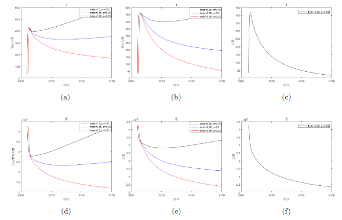
为了进行数值模拟, 我们需要对模型中的参数做出合理的估计. 其中人口的增长量, 患者的治愈率以及家畜的总量、屠宰率等相关数据主要参考全国第七次人口普查的结果与西藏统计年鉴, 而感染系数 $\beta_{1}, \beta_{2}, \beta_{3}$ 主要参考文献[13]. 而宣传教育产生的影响系数 $p$ , 流浪犬的环境最大容纳量 $K$ 以及归置率系数 $\theta$ 不易获得, 均为估计值. 具体数值如表2 所示.

根据公开发表的文献和公共卫生科学数据中心统计的包虫病病例可知, 西藏自治区从 2004-2020 年全区共报告病例数 1474 例, 其中 2017 年病例数最多为 273 例. 而 2012-2016 年完成的包虫病流行病学调查则显示西藏地区的包虫病患病率高达 1.66%, 之后完成的关于包虫病的普查工作, 进一步精确了西藏地区包虫病的患病率为 0.91%, 即我们模型中的潜伏期患者 $H_{e}$ . 由于西藏地区报告的病例数与当地实际的患病人数存在不相符的情况^[4], 所以我们在具体分析模拟结果时, 不仅要观察 $H_{i}$ 更应该关注 $H_{e}$ 的变化趋势.

下面我们利用 2012 年的数据 $H_{s}$ =3033666, $H_{e}$ =42500, $H_{i}$ =34, $D_{s}$ =2.38 $\times$ 10⁵, $D_{i}=7.2\times10^{4}$ , $L_{s}=2.53\times10^{7}$ , $L_{i}=3.683\times10^{6}$ 作为初始值条件进行计算. 其结果如图3-5 所示, 可以看出 $H_{i}$ 在 2016 年左右会达到峰值, 之后便会下降, 并且最大值不超过 450 例, 整体的变化趋势与实际情况是一致的. 此外将 $H_{e}$ 的模拟结果与文献[5]中西藏实际患病人数(见表1)比较可知, 除 2020 年的数据外, 另外四年的数据与模拟解之间匹配良好并且在稳步地减少. 这说明模型基本上符合当地的实际情况, 具有一定的合理性.

图3

图3 西藏地区 2016-2020 年实际患病人数与 $H_{e}$ 的比较

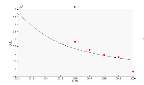
图4

图4 西藏地区未来 $50$ 年 $H_{e}$ 的变化趋势

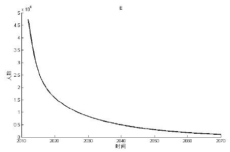
图5

图5 西藏地区未来 $50$ 年 $H_{i}$ 的变化趋势

表1 2016-2020西藏自治区人间包虫病患病率

新窗口打开| 下载CSV

表2 参数及参数值(单位:年)

新窗口打开| 下载CSV

4.2 防控策略讨论

下面我们研究 $p$ 和 $\theta$ 对基本再生数 $R_{0}$ 的影响, 进而讨论这两种防控措施. 令 $R_{0}=1, P, \theta$ 为参数, 可得

$p=1-\sqrt{\frac{bd(d_{l}+\varepsilon)(b_{d}-d)}{\beta_{2}\beta_{3}\varepsilon MK(b_{d}-d-\theta)}}:=p(\theta).$

即图6, 它刻画了宣传教育与流浪犬归置对基本再生数 $R_{0}$ 的影响, 当参数取值落在曲线的右上方区域时 $R_{0}<1$ , 疾病可控; 相反, 落在曲线左下方区域时 $R_{0}>1$ , 疾病得不到有效的控制.

图6

图6 $R_{0}=1$ 其中 $p, \theta$ 为参数的临界曲线

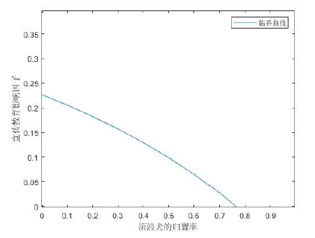
通过图像可知, 如果没有了平时的宣传教育, 即 $p=0$ 时, 要使 $R_{0}<1$ 则流浪犬的归置率 $\theta$ 需达到 75% 以上,这几乎是不可能的, 并且经济成本太大. 同理, 如果 $\theta=0$ 则需 $p>0.225$ , 这需要当地群众对包虫病的传播及预防有一个很高的认知. 但根据文献[17] 的调查, 2020 年中国西部五省(区)农牧民对包虫病防控相关知识的总知晓率仅为 57%, 而对包虫病感染途径的知晓率只有 30.8%. 因此, 以现阶段藏区群众的认知能力还不能达到如此效果. 这从侧面也说明了, 虽然近几年藏区患病人数在不断下降, 但防治成果还是很脆弱的, 为了能够使疾病继续保持一种下行的趋势, 两种防治措施还得同时实施, 如图 7 所示. 并且在未来很长的一段时间内, 在保持对流浪犬高归置率的同时(35%以上)还需加大宣传力度, 特别是针对一些重点人群的宣传, 比如一些远离聚集地, 年龄较大的农牧民, 因为这一部分群众接受信息的渠道少, 文化水平低, 但同时又处在最容易被感染的第一线. 未来随着整个地区群众对包虫病的认知能力都提高到一定程度后, 则可以逐步降低对流浪犬的归置率.

图7

图7 犬的归置率 $\theta$ 与宣传教育因素 $p$ 对疾病流行的影响

5 结论

本文根据包虫病的传播机理以及西藏地区的政策法规, 构建了一类符合西藏地区实际情况的包虫病动力学模型. 通过对模型的分析和应用, 发现当基本再生数 $R_{0}<1$ 时, 模型存在一个无病平衡点和一个平凡平衡点, 不存在地方病平衡点, 并且平凡平衡点总是不稳定的, 无病平衡点全局渐进稳定; 当 $R_{0}>1$ 时, 模型存在地方病平衡点并且全局渐近稳定. 利用表 1 中的数据可得 $R_{0}=0.96904$ , 即西藏地区的包虫病正在逐渐消亡, 模型模拟的结果与实际传播情况相符合. 最后讨论了宣传教育和对流浪犬归置两种防治措施对包虫病传播的影响, 结果表明, 两种措施必须同时施行才能达到控制疾病的目的, 并且由于现阶段藏区人民对包虫病的知晓率还比较低, 所以对流浪犬的归置率应一直保持高水平, 同时还要加大宣传力度, 当人们的预防意识有所提高后, 可逐步减少对流浪犬的归置.

参考文献

原文顺序

文献年度倒序

文中引用次数倒序

被引期刊影响因子

[1]

Eckert

, Deplazes

Biological, epidemiological, and clinical aspects of echinococ-cosis, a zoonosis of increasing concern

Clin Microbiol Rev, 2004, 17(1): 107-135

DOI:10.1128/CMR.17.1.107-135.2004 URL [本文引用: 1]

[2]

Davidson

R K

, Romig

, Jenkins

, et al.

The impact of globalisation on the distribution of Echinococcus multilocularis

Trends Parasitol, 2012, 28(6): 239-247

DOI:10.1016/j.pt.2012.03.004 PMID:22542923 [本文引用: 1]

In the past three decades, Echinococcus multilocularis, the cause of human alveolar echinococcosis, has been reported in several new countries both in definitive hosts (canids) as well as in people. Unless treated, infection with this cestode in people is fatal. In previously endemic countries throughout the Northern Hemisphere, geographic ranges and human and animal prevalence levels seem to be increasing. Anthropogenic influences, including increased globalisation of animals and animal products, and altered human/animal interfaces are thought to play a vital role in the global emergence of this pathogenic cestode. Molecular epidemiological techniques are a useful tool for detecting and tracing introductions, and differentiating these from range expansions.Copyright © 2012 Elsevier Ltd. All rights reserved.

[3]

陈伟奇, 张雅兰, 贡桑曲珍, 等.

西藏自治区棘球蚴病病例分析

中国寄生虫学与寄生虫病杂志, 2018, 36(1): 43-46

Chen

W Q

, Zhang

Y L

, GongSang

Q Z

, et al.

Analysis of hydatid disease cases in Tibet Autonomous Region

Chinese Journal of Parasitology and Parasitic Diseases, 2018, 36(1): 43-46

[4]

韩帅, 蒉嫣, 薛垂召, 等.

2004-2020年全国棘球蚴病疫情分析

中国寄生虫学与寄生虫病杂志, 2021, 39(5): 1-6

Han

, Kuai

, Xue

C Z

, et al.

The endemic status of echinococcosis in China from 2004 to 2020

Chinese Journal of Parasitology and Parasitic Diseases, 2021, 39(5): 1-6

[5]

蒉嫣, 伍卫平, 韩帅, 等.

2018-2019年全国棘球蚴病监测分析

中国病原生物学杂志, 2021, 16(9): 1025-1029

Kuai

, Wu

W P

, Han

, et al.

Analysis of the results of echinococcosis surveillance in China from 2018 to 2019

Journal of Pathogen Biology, 2021, 16(9): 1025-1029

[6]

Gemmell

M A

, Lawson

J R

, Roberts

M G

Population dynamics in echinococcosis and cysticercosis: biological parameters of Echinococcus granulosus in dogs and sheep

Parasitology, 1986, 92(3): 599-620

DOI:10.1017/S0031182000065483 URL [本文引用: 1]

The numerical distributions of Echinococcus granulosus in an experimental dog population are described. At all dose rates of protoscoleces from 10 to 175000 the distribution of worms was over-dispersed. Host age had no effect. There was a direct proportionality between the infective-stage density and rate of infection, and between the latter and the index of clumping. The worm burdens were significantly higher in the proximal than distal portions of the small intestine. Lengths of the 3- and 4-segmented worms increased from 4 to 10 and 4 to 8 weeks of age, respectively. Thereafter apolysis was asynchronous and could not be determined. Eggs were first detected in the faeces at 6 weeks and the mean age at oogenesis was 7·26 weeks. Retarded growth of the whole population of worms was observed in some dogs. For the first few infections, worm burdens varied widely in the same dog, but by the 6th infection 50% of the dog population had developed a relative insusceptibility to infection. Growth or oogenesis of the worms were not affected. A short-acting immune response was artificially induced in some dogs following the parenteral injection of activated embryos of E. granulosus, Taenia hydatigena, T. ovis, T. multiceps, T. pisiformis and T. serialis. The response affected either the number of worms established, growth or oogenesis or all three parameters. There was a strong positive correlation between numbers and lengths of worms in dogs with acquired and induced immunity, indicating that no ‘crowding’ effects were involved. In sheep populations the mean number of cysts which established was directly proportional to the number of eggs given, implying that there was no negative feedback mechanism operating at this stage of the life-cycle. The distribution of the larval population in sheep was over-dispersed and the index of clumping increased with the size of the egg dose from 25 to 2500 eggs. Protoscoleces were first observed in cysts at 2 years and the proportion producing them increased with age, with an estimate of 50% of cysts containing protoscoleces at 6 years. No deaths were observed in dogs or sheep even when high parasite burdens were present, implying that E. granulosus does not regulate the population of its hosts.

[7]

Roberts

M G

, Lawson

J R

, Gemmell

M A

Population dynamics in echinococcosis and cysticercosis: mathematical model of the life-cycle of Echinococcus granulosus

Parasitology, 1986, 92(3): 621-641

DOI:10.1017/S0031182000065495 URL [本文引用: 1]

A mathematical model of the life-cycle of Echinococcus granulosus in dogs and sheep in New Zealand is constructed and used to discuss previously published experimental and survey data. The model is then used to describe the dynamics of transmission of the parasite, and the means by which it may be destabilized. It is found that under the conditions that prevailed in New Zealand during the late 1950s, at the time of surveys of this parasite, the dog–sheep life-cycle was not regulated by any effective density-dependent constraint. In contrast there was evidence for an effective acquisition of immunity to reinfection by cattle. The long time to maturity of the cyst in sheep, together with the practice of feeding aged sheep to dogs, provides a time delay in the intermediate host. By comparison, the time to maturity of the adult stage in dogs is short, but it is of sufficient magnitude to be a key factor in the destabilization of the system by a regular dog-dosing programme. The model used to describe the life-cycle is a linear integrodifferential equation of the Volterra type. Such equations are intrinsically unstable in that a small perturbation in parameters can drive a previous equilibrium solution to zero. At the time of the surveys, the value of the basic reproductive rate, R0 was close to 1, and it has since been reduced below 1 by control measures.

[8]

杜守洪, 王蕾, 张学良, 等.

一类具有饱和发生率的包虫病传播模型研究

数学的实践与认识, 2013, 43(20): 269-273

S H

, Wang

, Zhang

X L

, et al.

A Echinococcosis model with saturation incidence

Journal of Mathematics in Practice and Theory, 2013, 43(20): 269-273

[9]

Liu

, Liu

, Feng

, et al.

Global dynamics of a time-delayed echinococcosis transmission model

Advances in Difference Equations, 2015, 2015(1): 1-16

DOI:10.1186/s13662-014-0331-4 URL [本文引用: 1]

[10]

, Ai

A spatial echinococcosis transmission model with time delays: stability and traveling waves

International Journal of Biomathematics, 2017, 10(6): 1-32

[11]

赵瑜, 杨诗杰.

一类随机包虫病传播模型及CDC数据拟合

生物数学学报, 2017, 32(1): 41-48

Zhao

, Yang

S J

Modeling a stochastic Echinococcosis transmission and fitting the statistical data of CDC

Journal of Biomathematics, 2017, 32(1): 41-48

[12]

Rong

X M

, Fan

, Sun

X D

, et al.

Impact of disposing stray dogs on risk assessment and control of Echinococcosis in Inner Mongolia

Mathematical Biosciences, 2018, 299: 85-96

DOI:S0025-5564(17)30436-4 PMID:29526551 [本文引用: 1]

Echinococcosis has been recognized as one of the most important helminth zoonosis in China. Available models always consider dogs as the mainly definitive hosts. However, such models ignore the distinctions between domestic dogs and stray dogs. In this study, we propose a 10-dimensional dynamic model distinguishing stray dogs from domestic dogs to explore the special role of stray dogs and potential effects of disposing stray dogs on the transmission of Echinococcosis. The basic reproduction number R, which measures the impact of both domestic dogs and stray dogs on the transmission, is determined to characterize the transmission dynamics. Global dynamic analysis of the model reveals that, without disposing the stray dogs, the Echinococcosis becomes endemic even the domestic dogs are controlled. Moreover, due to the difficulties in estimating the parameters involved in R with real data and the limitation of R in real-world applications, a new risk assessment tool called relative risk index I is defined for the control of zoonotic diseases, and the studies of the risk assessment for Echinococcosis infection show that it is essential to distinguish stray dogs from domestic dogs in applications.Copyright © 2018 Elsevier Inc. All rights reserved.

[13]

Wang

, Zhang

, Jin

, et al.

Modeling and analysis of the transmission of Echinococcosis with application to Xinjiang Uygur Autonomous Region of China

Journal of Theoretical Biology, 2013, 333: 78-90

DOI:10.1016/j.jtbi.2013.04.020 PMID:23669505 [本文引用: 2]

Echinococcosis, which is one of the zoonotic diseases, can threaten human health and hinder the development of animal husbandry seriously. Especially in Xinjiang Uygur Autonomous Region of China, Echinococcosis is regarded as one of the most serious endemic diseases.The number of human Echinococcosis has increased dramatically in the last 10 years, partially due to poor understanding of the transmission dynamics of Echinococcosis and lack of effective control measures of the disease. In this paper, in order to explore effective control and prevention measures we propose a deterministic model to study the transmission dynamics of Echinococcosis in Xinjiang. The results show that the dynamics of the model is completely determined by the basic reproductive number R0. If R0<1, the disease-free equilibrium is globally asymptotically stable. When R0>1, the disease-free equilibrium is unstable, and the endemic equilibrium is globally asymptotically stable. Based on the data reported by Xinjiang Center for Disease Control and Prevention (Xinjiang CDC), the numerical simulation result matches Echinococcosis data well. The model provides an approximate estimate of the basic reproduction number R0=1.67. This indicates that Echinococcosis is endemic in Xinjiang with the current control measures. Finally, we perform some sensitivity analysis of several model parameters and give some useful comments on controlling the transmission of Echinococcosis. Copyright © 2013 Elsevier Ltd. All rights reserved.

[14]

唐丹丹

新疆地区包虫病模型的建立与仿真

乌鲁木齐: 新疆医科大学, 2016

Tang

D D

The Establishment and Simulation of Echinococcosis Model in Xinjiang

Urumqi: Xinjiang Medical University, 2016

[15]

Zhang

, Xiao

Modeling and analyzing the effects of fixed-time intervention on transmission dynamics of echinococcosis in Qinghai province

Mathematical Methods in the Applied Sciences, 2018, 76: 1249-1267

[16]

Dreessche

, Watmough

Reproduction numbers and sub-threshold endemic equilibria for compartmental models of disease transmission

Mathematical Biosciences, 2002, 180: 29-48

PMID:12387915 [本文引用: 1]

A precise definition of the basic reproduction number, R0, is presented for a general compartmental disease transmission model based on a system of ordinary differential equations. It is shown that, if R0<1, then the disease free equilibrium is locally asymptotically stable; whereas if R0>1, then it is unstable. Thus, R0 is a threshold parameter for the model. An analysis of the local centre manifold yields a simple criterion for the existence and stability of super- and sub-threshold endemic equilibria for R0 near one. This criterion, together with the definition of R0, is illustrated by treatment, multigroup, staged progression, multistrain and vector-host models and can be applied to more complex models. The results are significant for disease control.

[17]

刘平, 吴海荣, 张伟超, 等.

我国西部地区农牧民包虫病防控认知情况及其影响因素

中国动物检疫, 2021, 38(5): 1-4

Liu

, Wu

H R

, Zhang

W C

, et al.

Awareness of herdsmen for the prevention and control of echinococcosis and potential risk factors in western china

China Animal Health Inspection, 2021, 38(5): 1-4