

1 引言与问题
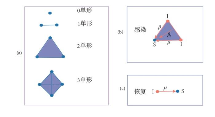
事实上, 真实世界中传染病的传播过程要更加复杂, 除了上述个体与个体间的接触之外, 还存在多元群体接触, 如家庭或工作场所中的接触, 也会对传染病的传播产生影响. 此情形下, 利用单纯复形网络可以很好地描述这种群体效应[10⇓-12]. 单纯复形网络是由单纯形构成, 一个
图1
受上述工作的启发, 基于模型 (1.1)[21]
其中
受随机因素的干扰, (1.2) 式中的参数
或
2 随机稳定性及随机分岔
2.1 随机稳定性
为了判断 (1.3) 式的随机稳定性, 可将其线性化之后依据线性 It
为了书写方便, 令
(1.3) 式变为
在 0 处线性化后 It
其中
类似可得到系统 (1.4) 的最大 Lyapunov 指数为
当最大 Lyapunov 指数小于 0 时, 线性化后的随机微分方程在 0 处依概率 1 渐进稳定, 系统的解趋近于无病平衡点. 对于系统 (1.3) 而言, 当
注 2.1 对比系统 (1.3) 和 (1.4), 可以发现, 噪声作用于一次项, 会改变确定性模型的基本再生数, 抑制疾病的暴发, 而噪声作用于高次项时, 则不改变确定性模型的基本再生数. 这是因为从量级上看,
2.2 随机分岔
系统 (2.2) 所对应的 Fokker-Planck 方程为
由此可求得稳态概率密度函数为
其中
显然
根据
(1) 若
(2) 若
同时, 从 (2.7) 式可看出
对于
(1) 当
(2) 当
(3) 当
类似对于
(1)
(2)
(3)
同理, 可得到系统 (1.4) 的稳态概率密度为
其中
3 数值模拟
图2
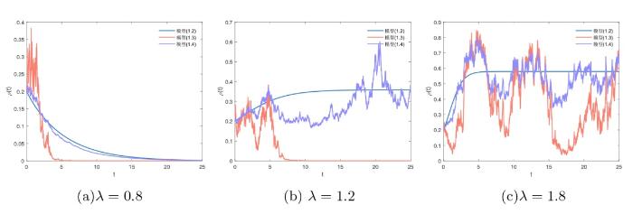
图2
根据上一章随机分岔的相关结果, 图3 分别给出了当
图3
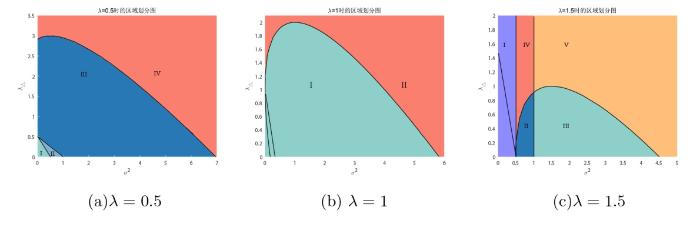
图3
图4
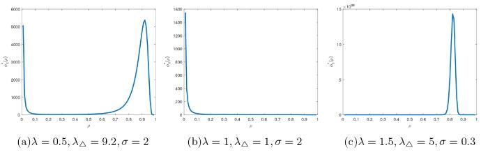
图5, 图6 及图7 分别给出了当
图5
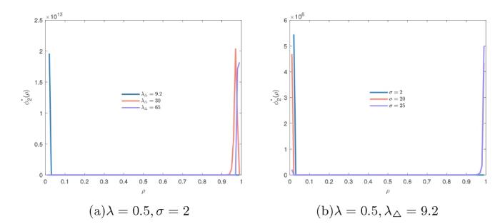
图6
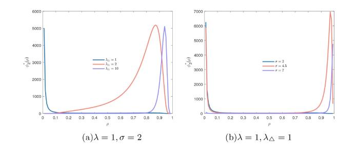
图7
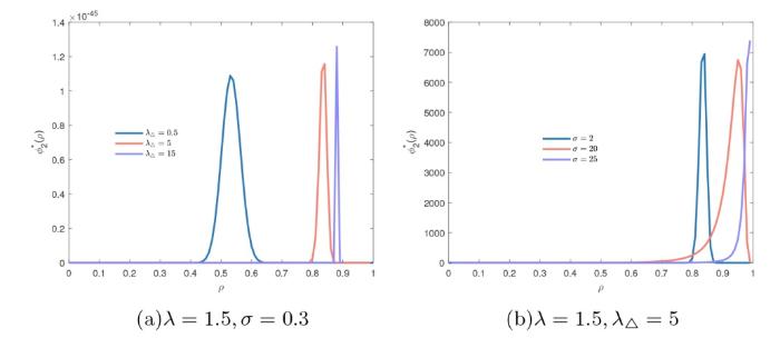
综上, 可以看出增大
4 结论
该文考虑了噪声影响下单纯复形上的 SIS 传染病模型, 比较了
参考文献
Collective dynamics of ‘small-world’networks
Emergence of scaling in random networks
DOI:10.1126/science.286.5439.509
PMID:10521342
[本文引用: 1]

Systems as diverse as genetic networks or the World Wide Web are best described as networks with complex topology. A common property of many large networks is that the vertex connectivities follow a scale-free power-law distribution. This feature was found to be a consequence of two generic mechanisms: (i) networks expand continuously by the addition of new vertices, and (ii) new vertices attach preferentially to sites that are already well connected. A model based on these two ingredients reproduces the observed stationary scale-free distributions, which indicates that the development of large networks is governed by robust self-organizing phenomena that go beyond the particulars of the individual systems.
Epidemic spreading in scale-free networks
The Internet has a very complex connectivity recently modeled by the class of scale-free networks. This feature, which appears to be very efficient for a communications network, favors at the same time the spreading of computer viruses. We analyze real data from computer virus infections and find the average lifetime and persistence of viral strains on the Internet. We define a dynamical model for the spreading of infections on scale-free networks, finding the absence of an epidemic threshold and its associated critical behavior. This new epidemiological framework rationalizes data of computer viruses and could help in the understanding of other spreading phenomena on communication and social networks.
Epidemic dynamics and endemic states in complex networks
Epidemic trajectories and awareness diffusion among unequals in simplicial complexes
Impact of simplicial complexes on epidemic spreading in partially mapping activity-driven multiplex networks
Epidemics on multilayer simplicial complexes
Simplicial models of social contagion
Competing spreading dynamics in simplicial complex
Cooperative epidemic spreading in simplicial complex
Simplicial SIS model in scale-free uniform hypergraph
Simplicial contagion in temporal higher-order networks
Comparison of deterministic and stochastic SIS and SIR models in discrete time
The asymptotic behaviour of a logistic epidemic model with stochastic disease transmission
The effect of loss of immunity on noise-induced sustained oscillations in epidemics
DOI:10.1007/s11538-011-9635-7
PMID:21347814
[本文引用: 1]
The effect of loss of immunity on sustained population oscillations about an endemic equilibrium is studied via a multiple scales analysis of a SIRS model. The analysis captures the key elements supporting the nearly regular oscillations of the infected and susceptible populations, namely, the interaction of the deterministic and stochastic dynamics together with the separation of time scales of the damping and the period of these oscillations. The derivation of a nonlinear stochastic amplitude equation describing the envelope of the oscillations yields two criteria providing explicit parameter ranges where they can be observed. These conditions are similar to those found for other applications in the context of coherence resonance, in which noise drives nearly regular oscillations in a system that is quiescent without noise. In this context the criteria indicate how loss of immunity and other factors can lead to a significant increase in the parameter range for prevalence of the sustained oscillations, without any external driving forces. Comparison of the power spectral densities of the full model and the approximation confirms that the multiple scales analysis captures nonlinear features of the oscillations.
A simple model for complex dynamical transitions in epidemics
DOI:10.1126/science.287.5453.667
PMID:10650003
[本文引用: 2]
Dramatic changes in patterns of epidemics have been observed throughout this century. For childhood infectious diseases such as measles, the major transitions are between regular cycles and irregular, possibly chaotic epidemics, and from regionally synchronized oscillations to complex, spatially incoherent epidemics. A simple model can explain both kinds of transitions as the consequences of changes in birth and vaccination rates. Measles is a natural ecological system that exhibits different dynamical transitions at different times and places, yet all of these transitions can be predicted as bifurcations of a single nonlinear model.
A multiplicative ergodic theorem. Characteristic Lyapunov, exponents of dynamical systems
