

1 引言
种群生态学主要是研究生物种群的数量与其栖息环境相互作用的科学, 是生态学领域的一个重要分支, 在理论上和方法上是生态学中最为发展、最为活跃的一个领域. 捕食-食饵模型作为一类研究种群动力学行为的模型, 成为了种群生态学的重要研究对象, 并得到了许多国内外学者的广泛关注, 取得了大量的研究成果[1⇓⇓⇓-5]. 1965 年, Holling[6] 在分析和实验的基础上, 研究了三种适应不同生物种群的功能反应函数. 2003 年, 陈兰荪等[7] 系统研究了具有第二类功能反应函数的捕食-食饵模型. 2016 年, Beroual 等[8] 研究了带有 Holling III 功能反应函数的捕食-食饵模型, 具体模型如下
其中
这里
其中
2 基础知识
下面先给出本文所用到的一些记号、定义及引理.
(1)
(2)
(3)
定义 2.1[16]
引理 2.1[16] (解的存在唯一性定理) 设
的解, 其中
则初始值为
引理 2.2[16] (
其中
引理 2.3[16] 设
引理 2.4[16] (随机微分方程比较定理) 设
的解, 其中
则有
引理 2.5[14] 设随机单种群模型
设
引理 2.6[17] 如果存在一个具有正则边界
则
3 主要结果
首先, 证明对任意给定正初始值, 系统 (1.3) 总是存在唯一的全局正解.
定理 3.1 任意给定的初始值
证 令
容易验证, 系统 (3.1) 满足局部 Lipschitz 条件和线性增长条件. 因此系统存在唯一的局部解
令
显然,
定义一个
利用
其中
由上式易得, 存在一个正常数
(3.2) 式两端从
令
或
根据 (3.3) 式可得
由于当
证毕.
然后, 我们给出系统
定理 3.2 设
证 对于系统
从而
其中
由上式可得, 存在一个正数
令
定理 3.3 设
证 设系统
由定理
故系统
下面我们讨论系统
定理 3.4 设
证
构造比较系统
由引理 2.4 和引理 2.5 可得, 当
利用
由
显然, 任意小的
由
由条件可知, 任意小的
同理, 利用
由
由条件可知, 任意小的
结合 (3.8) 及 (3.13) 式, 可得
由引理 2.3 可得
由
任意小的
由
任意小的
综上, 定理得证.
最后, 我们讨论系统的长期行为, 即系统在满足条件下的遍历性.
定理 3.5 设
证 定义李雅普诺夫函数
其中
其中
这里
由
选择足够小的正数
考虑下面的有界集
令
显然,
当
当
当
当
由上述情况可知, 对于任意的
此外, 设常数
综上, 由引理 2.6 可得, 系统 (1.3) 存在平稳分布, 并且此平稳分布具有遍历性. 证毕.
4 结论与数值模拟
文章研究了具有恐惧效应下的随机捕食-食饵系统, 利用随机分析的方法, 证明了系统对任意给定正初始值, 存在唯一的全局正解, 且满足均值有界性、随机最终有界性. 在满足一定条件下, 给出了系统食饵种群和捕食者种群灭绝和平均持续生存的充分条件, 并证明了系统存在平稳分布且具有遍历性. 为了验证上述结果的正确性, 我们采用 Milstein 方法, 对系统 (1.3) 进行数值模拟.
取
图1
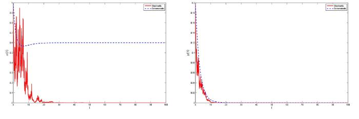
图1
系统 (1.3) 及其确定性系统的解. 其中
取
图2
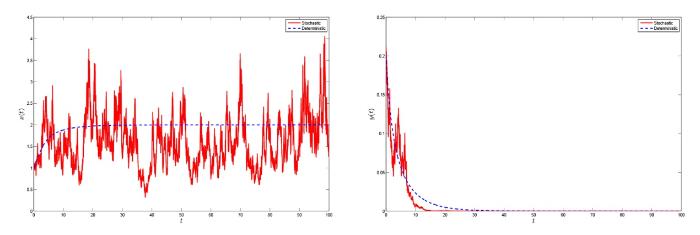
图2
系统 (1.3) 及其确定性系统的解. 其中
取
图3
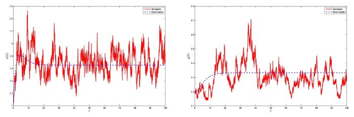
图3
系统 (1.3) 及其确定性系统的解. 其中
取
图4
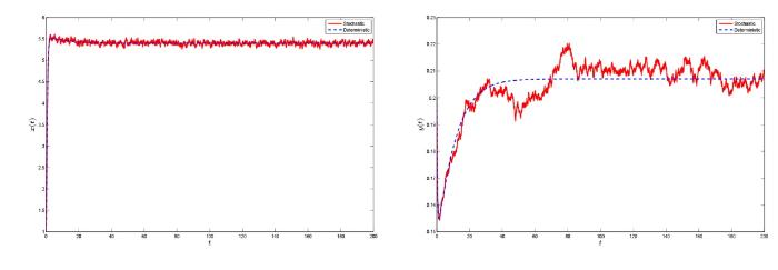
图4
系统 (1.3) 及其确定性系统的解. 其中
图5 给出了不同恐惧效应水平
图5
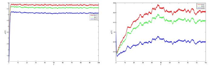
图5
不同恐惧效应水平对系统 (1.3) 解的影响. 其中
参考文献
Dynamics of a stochastic predator-prey model with fear effect and hunting cooperation
DOI:10.1007/s12190-022-01746-7 [本文引用: 1]
Stationary distribution and global stability of stochastic predator-prey model with disease in prey population
Dynamical complexity of a predator-prey model with a prey refuge and Allee effect
Dynamical behavior of a one-prey two-predator model with random perturbations
Dynamics of prey predator with Holling interactions and stochastic influences
The functional response of predators to prey density and its role in mimicry and population regulation
On a predator-prey system with Holling functional response:
Modelling the fear effect in predator-prey interactions

A recent field manipulation on a terrestrial vertebrate showed that the fear of predators alone altered anti-predator defences to such an extent that it greatly reduced the reproduction of prey. Because fear can evidently affect the populations of terrestrial vertebrates, we proposed a predator-prey model incorporating the cost of fear into prey reproduction. Our mathematical analyses show that high levels of fear (or equivalently strong anti-predator responses) can stabilize the predator-prey system by excluding the existence of periodic solutions. However, relatively low levels of fear can induce multiple limit cycles via subcritical Hopf bifurcations, leading to a bi-stability phenomenon. Compared to classic predator-prey models which ignore the cost of fear where Hopf bifurcations are typically supercritical, Hopf bifurcations in our model can be both supercritical and subcritical by choosing different sets of parameters. We conducted numerical simulations to explore the relationships between fear effects and other biologically related parameters (e.g. birth/death rate of adult prey), which further demonstrate the impact that fear can have in predator-prey interactions. For example, we found that under the conditions of a Hopf bifurcation, an increase in the level of fear may alter the direction of Hopf bifurcation from supercritical to subcritical when the birth rate of prey increases accordingly. Our simulations also show that the prey is less sensitive in perceiving predation risk with increasing birth rate of prey or increasing death rate of predators, but demonstrate that animals will mount stronger anti-predator defences as the attack rate of predators increases.
Effects of fear and additional food in a delayed predator-prey model
Role of fear in a predator-prey model with Beddington-DeAngelis functional response
Dynamics of a stochastic delay predator-prey model with fear effect and diffusion for prey
具有 Holling III 功能性反应的随机捕食食饵模型的平稳分布和周期解
Stationary distribution and periodic solution for stochastic predator-prey model with Holling-type III functional response
具有时滞和扩散的随机捕食-食饵系统
A stochastic predator-prey system with time delay and prey dispersal
随机环境下 Holling III 型捕食-食饵系统动力学行为
Dynamics behavior of the Holling III type predator-prey model in a random environment
Stochastic persistence and stationary distribution in a Holling-Tanner type prey-predator model
