1 引言
随着科技水平的提升, 我们所面临的许多实际问题也变得相对复杂, 而有些问题转化为积分方程的表达形式更容易被解决. 例如:金融数学、医学领域、化学和电化学过程[1 ,2 ] 、 电磁和电动力学、流体力学、生物学以及人口问题等等[3 ,4 ] . 其中 Volterra 型方程是积分方程的一种常见形式, 这类方程常被应用在流行病学的传播、种群遗传学、天线合成问题、人口动力学、半导体器件等[5 ⇓ ⇓ -8 ] 相关领域. 因此, 深入研究 Volterra 型积分方程, 对于解决以上实际问题具有重要意义, 例如以下第二类线性 Volterra 积分方程[5 ]
(1.1) $\begin{equation}\label{eq:1} g(x)-\mu \int^t_af(x,t)g(t){\rm d}t=w(x),\;\;x\in[a,b], \end{equation}$
其中 $\mu$ $w(x)\in L^{2}[a,b]$ $f(x,t) \in L^{2}([a,b])^{2}$ $g(x)$
由于此类方程对于工程中许多问题的建模非常重要, 所以解析方法和数值方法在分析此类模型并获得近似解方面发挥着重要作用[9 ⇓ ⇓ ⇓ ⇓ ⇓ ⇓ -16 ] . Abaoub 等人[9 ] 用定理证明了第二类线性和非线性 Volterra 积分方程解的存在唯一性. 曾[10 ] 理论分析了 Volterra 积分微分方程解的稳定性. 袁[11 ] 等人讨论了 Lotka-Volterra 竞争模型解的存在性. Chu[12 ] 给出了第二类线性 Volterra 积分方程解的存在性和唯一性的证明, 通过图像展示了所提出的最优同调渐近数值技术的可靠性和准确性. Khidir[13 ] 介绍了一种将 Volterra 积分方程转化为易于求解的代数方程组的切比雪夫谱配点法. Bulaic[14 ] 提供了一个 MatLab 工具箱,其主要目的是利用 MatLab 函数来求解第二类 Volterra 积分方程. 冯[15 ] 等人基于 Legendre 配置方法得到 Volterra 积分方程的数值解, 并给出严格的收敛性分析. Hesameddini 和 Shahbazi[16 ] 提出了一种基于移位标准正交 Bernstein 多项式的求解 Volterra-Fredholm 的可靠算法, 通过实例验证了该方法比 Legendre 配置法、泰勒配置法、泰勒多项式配置法和 Lagrange 配置法四种经典算法更有效.
本文将结合最小二乘法和再生核法来解决第二类 Volterra 型积分方程问题. 最小二乘法是计算数学中最基本的算法之一, 常常用来解决实际问题. 例如: Varah[17 ] 用最小二乘法来求解微分方程中出现参数的数值问题, 并从化学和生物建模的问题方面来说明该方法. Wang 等人[18 ] 利用最小二乘法估计指数律、对数律和复合函数模型的参数, 并进行各种拟合优度检验为小型风力发电机组的精确微观选址提供了依据. Rahman 等人[19 ] 采用稳健最小二乘法分析了各变量的边际效应, 来估计控制腐败对汇款流入有积极影响, 政府效率和政治稳定则会影响孟加拉国的汇款流入. 最小二乘法的其他应用详见文献 [20 ⇓ ⇓ ⇓ ⇓ -25 ]. 近年来, 再生核方法的应用也很广泛. 例如: 一般的一维界面问题[26 ] , 非局部分数阶边值问题[27 ] , 线性边值问题[28 ] , 三阶三点边值问题[29 ] , 非线性奇异边值问题[30 ] , 分数阶 Riccati 微分方程[31 ] , 具有周期边界条件的二阶微分方程组[32 ] , 非线性 Hamiltonian 系统[33 ] , 分数阶非线性微分方程[34 ] , 一维时滞传导方程[35 ] , Allen-Cahn 方程[36 ] 等相关问题都可以由再生核数值算法来求解.
本文的主要目的是在再生核空间 ${W}^m_{2}[a,b]$ $\varepsilon$
2 预备知识
本节介绍了再生核空间的相关知识点, 并且构造了一组再生核空间 ${W}^m_{2}[a,b]$
定义 2.1 [37 ] ${W}^m_{2}[a,b]=\{g(x)|g^{(m-1)}(x) \; \mbox{在}\; [a,b] \;\mbox{上是绝对连续的实值函数}, \;g^{(m)}(x) \in L^{2}[a,b]\}$ 是具有再生核 $K(x,y)$
(2.1) $\left\{\begin{array}{l} \langle g, h\rangle_{W_{2}^{m}[a, b]}=\sum_{j=1}^{m-1} g^{(j)}(a) h^{(j)}(a)+\int_{a}^{b} g^{(m)} h^{(m)} \mathrm{d} x, \quad g, h \in W_{2}^{m}[a, b] \\ \|g\|_{W_{2}^{m}[a, b]}=\sqrt{\langle g, g\rangle_{W_{2}^{m}[a, b]}}. \end{array}\right.$
为了方便, 把 $\langle \cdot,\cdot\rangle_{W^m_2[a,b]}$ $\left\|\cdot\right\|_{W^m_{2}[a,b]}$ $\langle \cdot,\cdot\rangle_m$ $\left\|\cdot\right\|_m$ $K_x^m(y)$ ${W}^m_{2}[a,b]$ $(\cdot,\cdot)$ $\left\|\cdot\right\|_0$ $L^{2}[a,b]$
引理 2.1 [37 ] 设 $H$ $H$ $X$
(1) $\forall x \in X$ $C_x$
(2) $\forall x \in X$ $K_x(y)\in H$
引理 2.2 对于 $\forall g \in W^m_{2}[a,b]$ $M$
下面, 我们将给出 $W^1_{2}[a,b]$
(2.2) $\begin{equation} \varphi_{s,j}=2^{\frac{s-1}{2}}\sqrt{b-a} \begin{cases} \frac{x-a}{b-a}-\frac{j}{2^{s-1}}, & x\in [\frac{j}{2^{s-1}}(b-a)+a,\frac{j+1/2}{2^{s-1}}(b-a)+a],\\[3mm] \frac{j+1}{2^{s-1}}-\frac{x-a}{b-a}, & x\in [\frac{j+1/2}{2^{s-1}}(b-a)+a,\frac{j+1}{2^{s-1}}(b-a)+a],\\ \quad 0, & \text {其他}. \end{cases} \end{equation}$
其中 $s=1,2,3,\cdots, j=0,1,\cdots,2^{s-1}-1$ .
引理 2.3 $\{1,\frac{x-a}{\sqrt{b-a}},\varphi_{1,0},\varphi_{2,0},\varphi_{2,1},\cdots,\varphi_{s,0},\varphi_{s,1},\cdots,\varphi_{s,2^{s-1}-1}, \cdots\}$ $W^1_{2}[a,b]$
证 首先, 证明这组基在 $W^1_{2}[a,b]$
下面, 证明这组基在 $W^1_{2}[a,b]$ $g\in W^1_{2}[a,b]$
只需证 $g\equiv0$ $\left\|\cdot\right\|_m$
由 $\{\frac{j}{2^{s-1}}(b-a)+a\}_{s,j}$ $[a,b]$ $g$ $g\equiv0$ . 基的完全性得证.
定义一个积分算子 $\mathcal{P}:L^{2}[a,b] \to C[a,b]$ $\forall g\in L^{2}[a,b]$ $\mathcal{P}g=\int^x_ag(t){\rm d} t$ . 则有如下两个引理
引理 2.4 $\{1,x-a,\frac{1}{2\sqrt{b-a}}(x-a)^{2},\mathcal{P}{\varphi_{1,0}},\mathcal{P}{\varphi_{2,0}},\mathcal{P}{\varphi_{2,1}},\cdots,\mathcal{P}{\varphi_{s,0}}, \mathcal{P}{\varphi_{s,1}},\cdots,\mathcal{P}{\varphi_{s,2^{s-1}-1}},$ $\cdots\}$ $W^2_{2}[a,b]$
使得 $g'\equiv0$ $g\equiv C$ $\langle 1,g\rangle_2=0$ $g\equiv0$
引理 2.5 $\{1,x-a,\frac{1}{2}(x-a)^{2},\frac{1}{6\sqrt{b-a}}(x-a)^{3},\mathcal{P}^{2}{\varphi_{1,0}},\mathcal{P}^{2}{\varphi_{2,0}},\mathcal{P}^{2}{\varphi_{2,1}},\cdots, \mathcal{P}^{2}{\varphi_{s,0}},\mathcal{P}^{2}{\varphi_{s,1}},$ $\cdots,\mathcal{P}^{2}{\varphi_{s,2^{s-1}-1}}, \cdots\}$ $W^3_{2}[a,b]$
下证基的完全性, 设 $g(x)\in W^3_{2}[a,b]$
由上可得 $g''\equiv0$ $g'\equiv C$ $\langle 1,g\rangle_3=\langle x-a,g\rangle_3=0$ $g(x)\equiv0$ . 证毕.
由此可见, 可以将上述得到的 $W^m_{2}[a,b]$
(2.3) $\begin{equation}\label{eq:a5} \{\psi_{j}\}^m_{j=0}\cup \{\phi_{s,0},\phi_{s,1},\cdots,\phi_{s,2^{s-1}-1}\}^\infty_{s=1}, \end{equation}$
3 算法及其收敛性分析
在这一节中, 我们针对方程 (1.1) 提出了一种基于最小二乘的新的再生核算法, 应用该算法得到了方程 (1.1) 的 $\varepsilon$
3.1 算子方程
定义一个算子 $\mathcal{A}:W^m_2[a,b] \to W^{m-2}_2[a,b]$ $f(x,t) \in C^{m}([a,b])^{2}$
引理 3.1 算子 $\mathcal{A}$
证 显然, 算子 $\mathcal{A}$
根据 $\left\|\cdot\right\|_{m}$
其中 $L_{1},L_{2},L_{3},L_{4}$
其中 $L$ $\mathcal{A}$
定义 3.1 $\forall \varepsilon >0$ $\exists v(x) \in W^{m}_2[a,b]$
则称 $v(x)$ $\varepsilon$
引理 3.2 设 $g(x)$ $g(x)\in W^{m}_2[a,b]$ $\forall \varepsilon >0$ $\varepsilon$
证 由于 $g(x)\in W^{m}_2[a,b]$ $g(x)$
这里 $p_{i}^{\star}=\langle \psi_{i},g\rangle_{m}$ $q_{s,j}^{\star}=\langle \phi_{s,j},g\rangle_{m}$ .
对 $\forall \varepsilon >0$ $\exists N$ $\forall n\geq N$
这里 $\left\|\mathcal{A}\right\|$ $\mathcal{A}$
故 $g_{n}^{\star}$ $\varepsilon$
3.2 算法
是方程 (1.1) 在 $W^{m}_2[a,b]$ $\varepsilon$
现要找到一组系数 $p_{0}^{\ast},p_{1}^{\ast},p_{2}^{\ast},\cdots,p_{m}^{\ast},q_{1,0}^{\ast},q_{2,0}^{\ast},q_{2,1}^{\ast}, \cdots,q_{n,0}^{\ast},q_{n,1}^{\ast},\cdots, q_{n,2^{n-1}-1}^{\ast}$
(3.1) $\begin{equation}\label{eq:2} \left\|\mathcal{A}g_{n}^{\ast}-w\right\|^{2}_m=\left\|\sum_{i=0}^{m}p_{i}^{\ast}\mathcal{A}\psi_{i} +\sum_{s=1}^{n}\sum_{j=0}^{2^{s-1}-1}q_{s,j}^{\ast}\mathcal{A}\phi_{s,j}-w\right\|^{2}_m=\min J, \end{equation}$
求算法 (3.1) 中的 $J$
(3.2) $\begin{equation}\label{eq:3} \begin{cases} \langle \mathcal{A}\psi_{i},\mathcal{A}g_{n}\rangle_m=\langle \mathcal{A}\psi_{i},w\rangle_m,\;i=0,1,2,\cdots,m,\\ \langle \mathcal{A}\phi_{s,j},\mathcal{A}g_{n}\rangle_m=\langle \mathcal{A}\phi_{s,j},w\rangle_m,\;s=1,2,\cdots,n, j=0,1,2,\cdots,2^{s-1}-1. \end{cases} \end{equation}$
由 (3.2) 式可得 $p_{0}^{\ast},p_{1}^{\ast},p_{2}^{\ast},\cdots,p_{m}^{\ast},q_{1,0}^{\ast},q_{2,0}^{\ast},q_{2,1}^{\ast}, \cdots,q_{n,0}^{\ast},q_{n,1}^{\ast},\cdots,q_{n,2^{n-1}-1}^{\ast}$
定理 3.1 由 (3.1) 式得到的近似解 $g_{n}^{\ast}(x)$ $\varepsilon$
这表明由 (3.1) 式得到的近似解 $g_{n}^{\ast}(x)$ $\varepsilon$
定理 3.2 设 $\mathcal{A}$ $W^m_2[a,b] \to W^{m-2}_2[a,b]$ $\varepsilon$
证 设 (3.2) 式的系数矩阵为 $G$ . 由于 $G$ $Gram$
是 $W^m_2[a,b]$
是线性无关的, 又由算子 $\mathcal{A}$
令 $\lambda$ $G$ $H=(h_{1},h_{2},\cdots,h_{N})^{T}$ $\left\|H\right\|_{0}=1$
这里 $\mathcal{A}^{-1}$ $\mathcal{A}$
则 $G$
3.3 算法分析
定理 3.3 设 $g^{\ast}_{n}(x)$ $\varepsilon$ $g^{\ast}_{n}(x)$ $[a,b]$ $g(x)$ .
又由算子 $\mathcal{A}$ $\mathcal{A}^{-1}$ $\left\|g-g_{n}^{\star}\right\|\rightarrow 0(n\rightarrow\infty)$
定理 3.4 设 $g(x)\in W^m_2[a,b]$ $g^{\ast}_{n}(x)$ $\varepsilon$
进而 $\left\|g-g^{\ast}_{n}\right\|_{m} \leq 2^{-n}M.$
在求解第二类非线性 Volterra 积分方程时, 需将第 3 节算法和拟牛顿法相结合. 首先, 利用拟牛顿法处理非线性模型中的非线性项, 将问题转化为线性模型. 再次, 应用最小二乘法将该线性模型转化为一个线性代数方程组进行求解, 进而得到原模型的 $\varepsilon$
4 数值算例
本节为了验证所提算法的精确性和适用性, 研究以下八个数值算例 (其中线性算例 1-4, 非线性算例 5-8), 并计算得到相应的误差和不同范数意义下的数值结果. 我们有如下定义
其中 $\mu=-1,$ $f(x,t)= x,$ $w(x)={\rm e}^{x}-x {\rm e}^{x} +\sin x+x \cos x,$
精确解 $g(x)={\rm e}^{x}+\sin x$ .
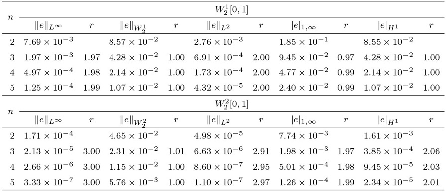
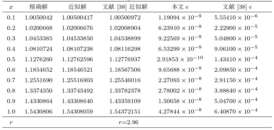
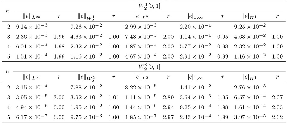
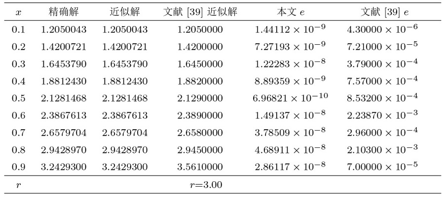
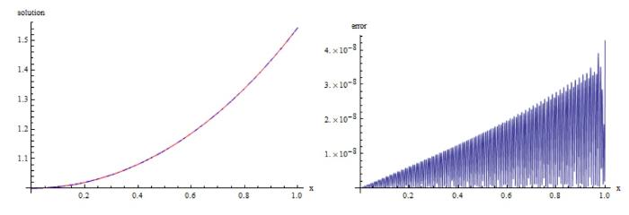
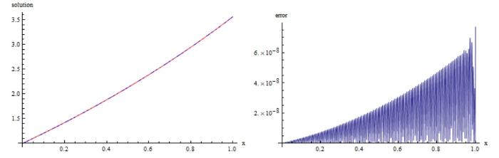
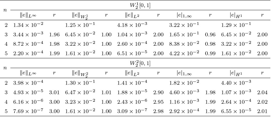
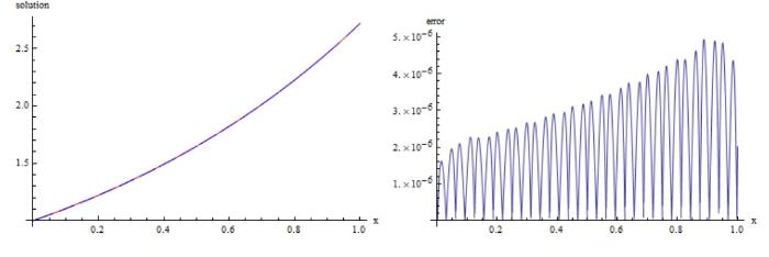
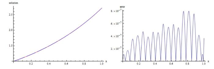
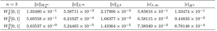
在表1 、3 中, 分别给出了算例 1、2 的 $\|e\|_{L^\infty}$ $\|e\|_{W^m_2}$ $\|e\|_{L^2}$ $|e|_{1,\infty}$ $|e|_{H^{1}}$ $\|e\|_{L^\infty}$ $\|e\|_{L^2}$ $W^m_2[a,b]$ 表2 、4 展示了应用我们的方法得到的误差与文献 [38 ,39 ] 的方法进行比较, 数值结果表明我们的方法更接近精确解. 另外, 在图1 、2 中展现了精确解和近似解及其误差.
图1
图1
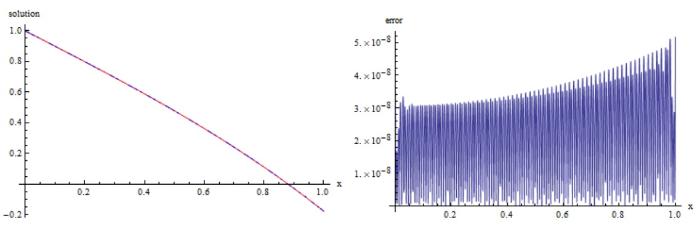
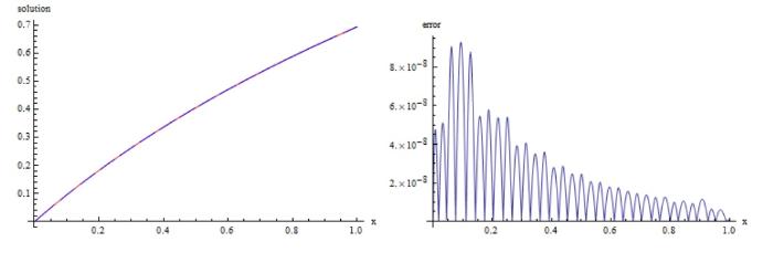
算例 1 左图: 红色为精确解, 蓝色为近似解; 右图: $|g(x)-g^{\ast}_{n}(x)|$
图2
图2
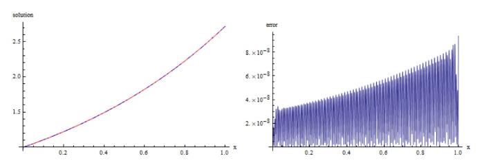
算例 2 左图: 红色为精确解, 蓝色为近似解; 右图: $|g(x)-g^{\ast}_{n}(x)|$
其中 $\mu=1$ $f(x,t)=x-t$ $w(x)=1-x-\frac{x^{2}}{2}$ $g(x)=1-\sinh x$ .
其中 $\mu=2$ $f(x,t)=\sin (x-t)$ $w(x)=\sin x +\cos x$ $g(x)=\sin x$ .
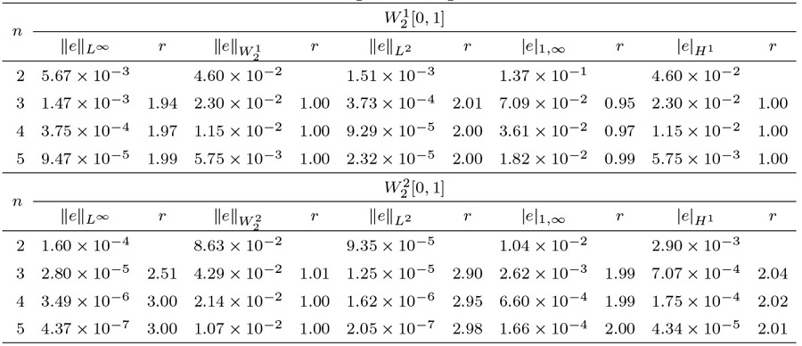
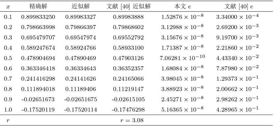
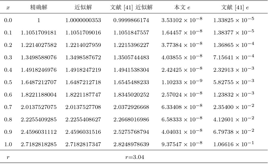
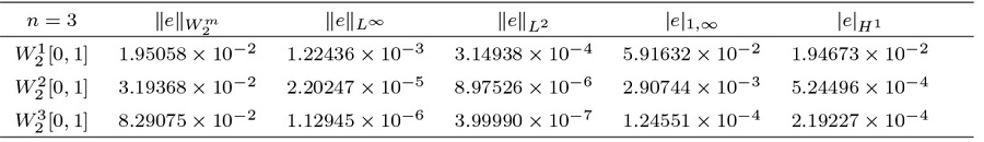
在表5 、7 中, 分别展示了算例 3、4 在 $W^1_2[a,b]$ $W^2_2[a,b]$ $\|e\|_{L^\infty}$ 表6 、8 表明应用我们的方法得到的结果, 并与文献 [40 ,41 ] 中方法进行比较, 数值结果验证了我们的方法更有效.
图3
图3
算例 3 左图: 红色为精确解, 蓝色为近似解; 右图: $|g(x)-g^{\ast}_{n}(x)|$
图4
图4
算例 4 左图: 红色为精确解, 蓝色为近似解; 右图: $|g(x)-g^{\ast}_{n}(x)|$
其中 $\mu=-1$ $f(x,t)={\rm e}^{(x-t)}, w(x)={\rm e}^{2x}$ $g(x)={\rm e}^{x}$ .
其中 $\mu=1$ $w(x)={\rm e}^{x}-\frac{1}{2}({\rm e}^{2x}-1)$ $g(x)={\rm e}^{x}$ .
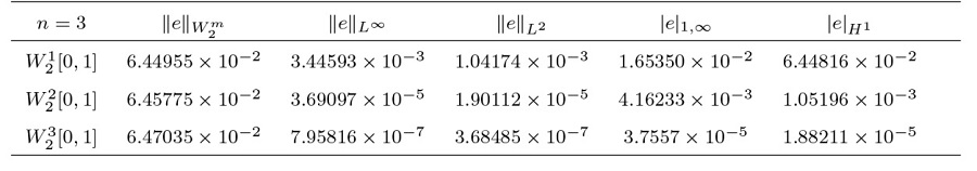
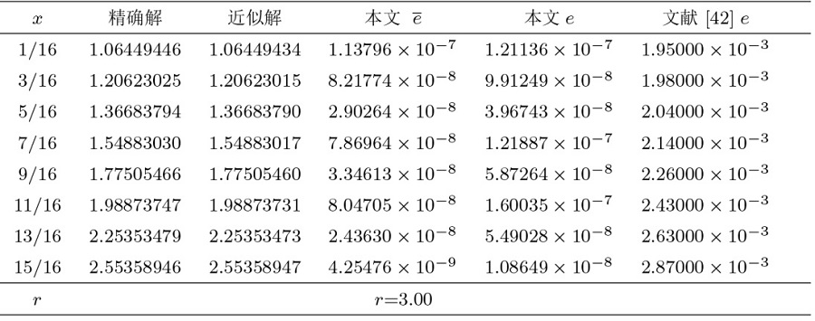
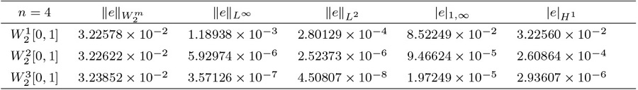
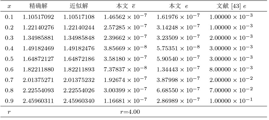
在表9 、11 中, 分别展示了算例 5、6 在 $W^m_2[a,b]$ 表10 、12 展示了应用我们的方法得到的误差与文献 [42 ,43 ] 中方法进行比较, 数值结果表明我们的方法更精确. 另外, 在图5 、6 中展现了精确解和近似解的拟合程度.
图5
图5
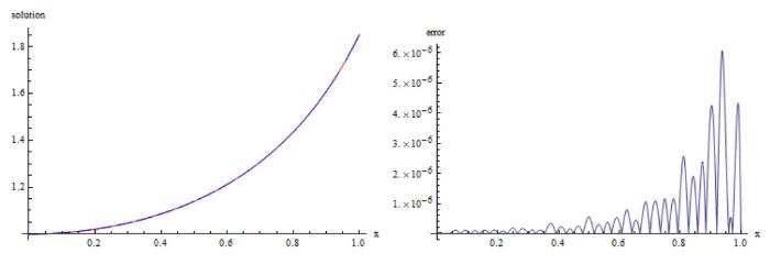
算例 5 左图: 红色为精确解, 蓝色为近似解; 右图: $|g(x)-g^{\ast}_{n}(x)|$
图6
图6
算例 6 左图: 红色为精确解, 蓝色为近似解; 右图: $|g(x)-g^{\ast}_{n}(x)|$
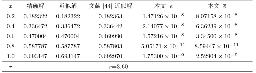
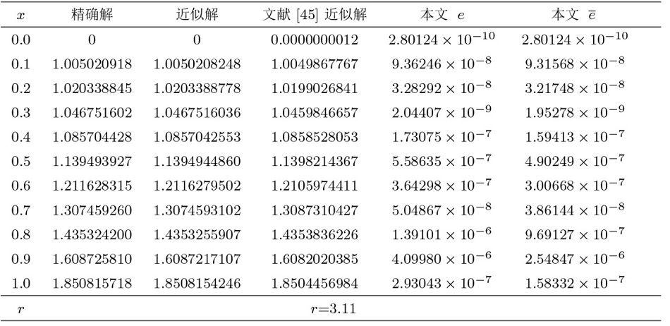
从表12 、15 分别可以得到算例 7 和 8 在 $W^m_2[a,b]$ 表13 、16 表明应用我们的方法得到的误差与文献 [44 ,45 ] 的方法进行比较, 数值结果验证了我们的方法是解决这类问题有效方法. 另外, 在图7 、8 中展现了精确解和近似解以及相对应的误差图像.
图7
图7
算例 7 左图: 红色为精确解, 蓝色为近似解; 右图: $|g(x)-g^{\ast}_{n}(x)|$
图8
图8
算例 8 左图: 红色为精确解, 蓝色为近似解; 右图: $|g(x)-g^{\ast}_{n}(x)|$
5 结论
本文基于最小二乘法提出了一种求解第二类 Volterra 型积分方程的再生核算法, 并理论分析了此方法得到的 $\varepsilon$
参考文献
View Option
[1]
Salon S Chari M Numerical Methods in Electromagnetism . Beijing : Academic Press , 1999
[本文引用: 1]
[3]
Chew W C Tong M S Hu B Integral Equation Methods for Electromagnetic and Elastic Waves . Berlin : Springer Nature , 2022
[本文引用: 1]
[4]
Bloom F Asymptotic bounds for solutions to a system of damped integro-differential equations of electromagnetic theory
J Math Anal Appl , 1980 , 73 2 ): 524 -542
[本文引用: 1]
[5]
Wazwaz A M Linear and Nonlinear Integral Equations . Berlin : Springer , 2011
[本文引用: 2]
[6]
Tang Q Waxman D An integral equation describing an asexual population in a changing environment
Nonlinear Anal , 2003 , 53 5 ): 683 -699
[本文引用: 1]
[7]
Corduneanu C Integral Equations and Applications . Cambridge : Cambridge University , Press , 1991
[本文引用: 1]
[8]
Schiavone P Constanda C Mioduchowski A Integral Methods in Science and Engineering . Boston : Birkhäuser , 2012
[本文引用: 1]
[9]
Abaoub A E Shkheam A S Zali S M The Adomian decomposition method of Volterra integral equation of second kind
Am J Appl Math , 2018 , 6 4 ): 142 -148
[本文引用: 2]
[10]
曾志刚 . Volterra 积分微分方程的稳定性
数学物理学报 , 2001 , 21A 1 ): 48 -54
[本文引用: 2]
Zeng Z G Stability of Volterra integro differential equations
Acta Math Sci , 2001 , 21A 1 ): 48 -54
[本文引用: 2]
[11]
袁海龙 , 李艳玲 . 一类具有 Lotka-Volterra 竞争模型共存解的存在性与稳定性
数学物理学报 , 2017 , 37A 1 ): 173 -184
[本文引用: 2]
Yuan H L Li Y L The existence and stability of coexistence solutions of a kind of Lotka-Volterra competition model
Acta Math Sci , 2017 , 37A 1 ): 173 -184
[本文引用: 2]
[12]
Chu Y M Ullah S Ali M et al . Numerical investigation of Volterra integral equations of second kind using optimal homotopy asymptotic method
Appl Math Comput , 2022 , 430 127304
[本文引用: 2]
[13]
Khidir A A A new numerical technique for solving Volterra integral equations using Chebyshev spectral method
Math Probl Eng , 2021 , 2021 1 -11
[本文引用: 2]
[14]
Bulai I M De Bonis M C Laurita C et al . MatLab Toolbox for the numerical solution of linear Volterra integral equations arising in metastatic tumor growth models
Dolomites Research Notes on Approximation , 2022 , 15 2 ): 13 -24
[本文引用: 2]
[15]
冯立新 , 杨晓旭 . 解带有扰动数据的第一类 Volterra 积分方程的谱正则化方法
数学物理学报 , 2020 , 40A 3 ): 650 -661
[本文引用: 2]
Feng L X Yang X X Spectral regularization method for solving Volterra integral equation of the first kind with perturbed data
Acta Math Sci , 2020 , 40A 3 ): 650 -661
[本文引用: 2]
[16]
Hesameddini E Shahbazi M A reliable algorithm based on the shifted orthonormal Bernstein polynomials for solving Volterra-Fredholm integral equations
Journal of Taibah University for Science , 2018 , 12 4 ): 427 -438
[本文引用: 2]
[17]
Varah J M A spline least squares method for numerical parameter estimation in differential equations
SIAM J Sci Comput , 1982 , 3 1 ): 28 -46
[本文引用: 1]
[18]
Wang W X Xu Y Han X L Gao M L et al . A study of function-based wind profiles based on least squares method: A case in the suburbs of Hohho
Energy Reports , 2022 , 8 4303 -4318
[本文引用: 1]
[19]
Rahman M H Habib A Impact of economic and noneconomic factors on inflow of remittances into bangladesh: Application of robust least squares method
Finance and Economics Review , 2021 , 3 1 ): 51 -62
[本文引用: 1]
[20]
张晶 , 余旌胡 . 线性回归模型参数估计方法的分辨率
数学物理学报 , 2020 , 40A 5 ): 1381 -1392
[本文引用: 1]
Zhang J Yu J H Parameter resolution of estimation methods for linear regression models
Acta Math Sci , 2020 , 40A 5 ): 1381 -1392
[本文引用: 1]
[21]
马奕佳 , 薛留根 , 芦飞 . 缺失数据下部分非线性变系数 EV 模型的统计推断
数学物理学报 , 2020 , 40A 2 ): 460 -474
[本文引用: 1]
Ma Y J Xue L g Lu F Statistical inference in partially nonlinear varying-coefficient Errors-Variables models with missing responses
Acta Math Sci , 2020 , 40A 2 ): 460 -474
[本文引用: 1]
[22]
冯三营 , 薛留根 , 范承华 . 非线性半参数回归模型中参数的经验似然置信域
数学物理学报 , 2009 , 29A 5 ): 1338 -1349
[本文引用: 1]
Feng S Y Xue L G Fan C H Empirical likelihood confidence regions of the parameters in nonlinear semiparametric regression models
Acta math sci , 2009 , 29A 5 ): 1338 -1349
[本文引用: 1]
[23]
Salehi R Dehghan M A generalized moving least square reproducing kernel method
J Comput Appl Math , 2013 , 249 120 -132
[本文引用: 1]
[24]
Liu G Han X Lam K Y A combined genetic algorithm and nonlinear least squares method for material characterization using elastic waves
Comput Methods Appl. Mech Engrg , 2002 , 191 17/18 ): 1909 -1921
[本文引用: 1]
[25]
Fonken J M Ramaswamy K R Paul M J A scalable multi-step least squares method for network identification with unknown disturbance topology
Automatica , 2022 , 141 110295
[本文引用: 1]
[26]
Sun L X Niu J Hou J J A high order convergence collocation method based on the reproducing kernel for general interface problems
Appl Math Lett , 2021 , 112 106718
[本文引用: 1]
[27]
Geng F Z Cui M G A reproducing kernel method for solving nonlocal fractional boundary value problems
Appl Math Lett , 2012 , 25 5 ): 818 -823
[本文引用: 1]
[28]
Li X Y Wu B Y Error estimation for the reproducing kernel method to solve linear boundary value problems
J Comput Appl Math , 2013 , 243 10 -15
[本文引用: 1]
[29]
Wu B Y Li X Y Application of reproducing kernel method to third order three-point boundary value problems
Appl Math Comput , 2010 , 217 7 ): 3425 -3428
[本文引用: 1]
[30]
Niu J Xu M Q Lin Y Z Xue Q Numerical solution of nonlinear singular boundary value problems
J Comput Appl Math , 2018 , 331 42 -51
[本文引用: 1]
[31]
Xu M Q Tohidi E Niu J Fang Y Z A new reproducing kernel-based collocation method with optimal convergence rate for some classes of BVPs
Appl Math Comput , 2022 , 432 127343
[本文引用: 1]
[32]
Al-Smadia M Arqub O A Shawagfeh N Momanic S Numerical investigations for systems of second-order periodic boundary value problems using reproducing kernel method
Appl Math Comput , 2016 , 291 137 -148
[本文引用: 1]
[33]
Niu J Jia Y T Sun J D A new piecewise reproducing kernel function algorithm for solving nonlinear Hamiltonian systems
Appl Math Lett , 2023 , 136 108451
[本文引用: 1]
[34]
Xu M Q Niu J Lin Y Z An efficient method for fractional nonlinear differential equations by quasi-Newton's method and simplified reproducing kernel method
Math Methods Appl Sci , 2018 , 41 1 ): 5 -14
[本文引用: 1]
[35]
Niu J Sun L X Xu M Q Hou J J A reproducing kernel method for solving heat conduction equations with delay
Appl Math Lett , 2020 , 100 106036
[本文引用: 1]
[36]
Niu J Xu M Yao G M An efficient reproducing kernel method for solving the Allen-Cahn equation
Appl Math Lett , 2019 , 89 78 -84
[本文引用: 1]
[37]
吴勃英 , 林迎珍 . 应用型再生核空间 . 北京 : 科学出版社 , 2012
[本文引用: 2]
Wu B Y Lin Y Z Applied Regenerative Nuclear Space . Beijing : Science Press , 2012
[本文引用: 2]
[38]
Babolian E Davari A Numerical implementation of Adomian decomposition method for linear Volterra integral equations of the second kind
Appl Math Comput , 2005 , 165 1 ): 223 -27
[本文引用: 2]
[39]
Dalal A M The modified decompositon method for solving Volterra integral equations of the second kind using Maple
Int J GEOMATE , 2019 , 17 62 ): 23 -28
[本文引用: 2]
[40]
Saad S Mushtaq A K B Some new applications of Elzaki transform for solution of linear Volterra type integral equations
J Appl Math Phys , 2019 , 7 8 ): 1877 -1892
[本文引用: 2]
[41]
Ahmet A Application of the Bernstein polynomials for solving Volterra integral equations with convolution kernels
Faculty of Sciences and Mathematics , 2016 , 30 4 ): 1045 -1052
[本文引用: 2]
[42]
Singh I Kumar S Haar wavelet method for some nonlinear Volterra integral equations of the first kind
J Comput Appl Math , 2016 , 292 541 -552
[本文引用: 2]
[43]
Babolian E Shahsavarani A Numerical solution of nonlinear Fredholm and Volterra integral equations of the second kind using Haar wavelets and collocation method
J Sci Tarbiat Moallem University , 2007 , 7 213 -222
[本文引用: 2]
[44]
Mahmoudi Y Wavelet Galerkin method for numerical solution of nonlinear integral equation
Appl Math Comput , 2005 , 167 1119 -1129
[本文引用: 2]
[45]
Ishola C Y Taiwo O A Adedokun K A et al . Solution of nonlinear Volterra integral equations by Chebyshev collocation approximation method
Pacific Journal of Science and Technology , 2022 , 23 1 ): 34 -39
[本文引用: 2]
1
1999
... 随着科技水平的提升, 我们所面临的许多实际问题也变得相对复杂, 而有些问题转化为积分方程的表达形式更容易被解决. 例如:金融数学、医学领域、化学和电化学过程[1 ,2 ] 、 电磁和电动力学、流体力学、生物学以及人口问题等等[3 ,4 ] . 其中 Volterra 型方程是积分方程的一种常见形式, 这类方程常被应用在流行病学的传播、种群遗传学、天线合成问题、人口动力学、半导体器件等[5 ⇓ ⇓ -8 ] 相关领域. 因此, 深入研究 Volterra 型积分方程, 对于解决以上实际问题具有重要意义, 例如以下第二类线性 Volterra 积分方程[5 ] ...
Quantum effects of thermal radiation in a Kerr nonlinear blackbody
1
2002
... 随着科技水平的提升, 我们所面临的许多实际问题也变得相对复杂, 而有些问题转化为积分方程的表达形式更容易被解决. 例如:金融数学、医学领域、化学和电化学过程[1 ,2 ] 、 电磁和电动力学、流体力学、生物学以及人口问题等等[3 ,4 ] . 其中 Volterra 型方程是积分方程的一种常见形式, 这类方程常被应用在流行病学的传播、种群遗传学、天线合成问题、人口动力学、半导体器件等[5 ⇓ ⇓ -8 ] 相关领域. 因此, 深入研究 Volterra 型积分方程, 对于解决以上实际问题具有重要意义, 例如以下第二类线性 Volterra 积分方程[5 ] ...
1
2022
... 随着科技水平的提升, 我们所面临的许多实际问题也变得相对复杂, 而有些问题转化为积分方程的表达形式更容易被解决. 例如:金融数学、医学领域、化学和电化学过程[1 ,2 ] 、 电磁和电动力学、流体力学、生物学以及人口问题等等[3 ,4 ] . 其中 Volterra 型方程是积分方程的一种常见形式, 这类方程常被应用在流行病学的传播、种群遗传学、天线合成问题、人口动力学、半导体器件等[5 ⇓ ⇓ -8 ] 相关领域. 因此, 深入研究 Volterra 型积分方程, 对于解决以上实际问题具有重要意义, 例如以下第二类线性 Volterra 积分方程[5 ] ...
Asymptotic bounds for solutions to a system of damped integro-differential equations of electromagnetic theory
1
1980
... 随着科技水平的提升, 我们所面临的许多实际问题也变得相对复杂, 而有些问题转化为积分方程的表达形式更容易被解决. 例如:金融数学、医学领域、化学和电化学过程[1 ,2 ] 、 电磁和电动力学、流体力学、生物学以及人口问题等等[3 ,4 ] . 其中 Volterra 型方程是积分方程的一种常见形式, 这类方程常被应用在流行病学的传播、种群遗传学、天线合成问题、人口动力学、半导体器件等[5 ⇓ ⇓ -8 ] 相关领域. 因此, 深入研究 Volterra 型积分方程, 对于解决以上实际问题具有重要意义, 例如以下第二类线性 Volterra 积分方程[5 ] ...
2
2011
... 随着科技水平的提升, 我们所面临的许多实际问题也变得相对复杂, 而有些问题转化为积分方程的表达形式更容易被解决. 例如:金融数学、医学领域、化学和电化学过程[1 ,2 ] 、 电磁和电动力学、流体力学、生物学以及人口问题等等[3 ,4 ] . 其中 Volterra 型方程是积分方程的一种常见形式, 这类方程常被应用在流行病学的传播、种群遗传学、天线合成问题、人口动力学、半导体器件等[5 ⇓ ⇓ -8 ] 相关领域. 因此, 深入研究 Volterra 型积分方程, 对于解决以上实际问题具有重要意义, 例如以下第二类线性 Volterra 积分方程[5 ] ...
... [5 ] ...
An integral equation describing an asexual population in a changing environment
1
2003
... 随着科技水平的提升, 我们所面临的许多实际问题也变得相对复杂, 而有些问题转化为积分方程的表达形式更容易被解决. 例如:金融数学、医学领域、化学和电化学过程[1 ,2 ] 、 电磁和电动力学、流体力学、生物学以及人口问题等等[3 ,4 ] . 其中 Volterra 型方程是积分方程的一种常见形式, 这类方程常被应用在流行病学的传播、种群遗传学、天线合成问题、人口动力学、半导体器件等[5 ⇓ ⇓ -8 ] 相关领域. 因此, 深入研究 Volterra 型积分方程, 对于解决以上实际问题具有重要意义, 例如以下第二类线性 Volterra 积分方程[5 ] ...
1
1991
... 随着科技水平的提升, 我们所面临的许多实际问题也变得相对复杂, 而有些问题转化为积分方程的表达形式更容易被解决. 例如:金融数学、医学领域、化学和电化学过程[1 ,2 ] 、 电磁和电动力学、流体力学、生物学以及人口问题等等[3 ,4 ] . 其中 Volterra 型方程是积分方程的一种常见形式, 这类方程常被应用在流行病学的传播、种群遗传学、天线合成问题、人口动力学、半导体器件等[5 ⇓ ⇓ -8 ] 相关领域. 因此, 深入研究 Volterra 型积分方程, 对于解决以上实际问题具有重要意义, 例如以下第二类线性 Volterra 积分方程[5 ] ...
1
2012
... 随着科技水平的提升, 我们所面临的许多实际问题也变得相对复杂, 而有些问题转化为积分方程的表达形式更容易被解决. 例如:金融数学、医学领域、化学和电化学过程[1 ,2 ] 、 电磁和电动力学、流体力学、生物学以及人口问题等等[3 ,4 ] . 其中 Volterra 型方程是积分方程的一种常见形式, 这类方程常被应用在流行病学的传播、种群遗传学、天线合成问题、人口动力学、半导体器件等[5 ⇓ ⇓ -8 ] 相关领域. 因此, 深入研究 Volterra 型积分方程, 对于解决以上实际问题具有重要意义, 例如以下第二类线性 Volterra 积分方程[5 ] ...
The Adomian decomposition method of Volterra integral equation of second kind
2
2018
... 由于此类方程对于工程中许多问题的建模非常重要, 所以解析方法和数值方法在分析此类模型并获得近似解方面发挥着重要作用[9 ⇓ ⇓ ⇓ ⇓ ⇓ ⇓ -16 ] . Abaoub 等人[9 ] 用定理证明了第二类线性和非线性 Volterra 积分方程解的存在唯一性. 曾[10 ] 理论分析了 Volterra 积分微分方程解的稳定性. 袁[11 ] 等人讨论了 Lotka-Volterra 竞争模型解的存在性. Chu[12 ] 给出了第二类线性 Volterra 积分方程解的存在性和唯一性的证明, 通过图像展示了所提出的最优同调渐近数值技术的可靠性和准确性. Khidir[13 ] 介绍了一种将 Volterra 积分方程转化为易于求解的代数方程组的切比雪夫谱配点法. Bulaic[14 ] 提供了一个 MatLab 工具箱,其主要目的是利用 MatLab 函数来求解第二类 Volterra 积分方程. 冯[15 ] 等人基于 Legendre 配置方法得到 Volterra 积分方程的数值解, 并给出严格的收敛性分析. Hesameddini 和 Shahbazi[16 ] 提出了一种基于移位标准正交 Bernstein 多项式的求解 Volterra-Fredholm 的可靠算法, 通过实例验证了该方法比 Legendre 配置法、泰勒配置法、泰勒多项式配置法和 Lagrange 配置法四种经典算法更有效. ...
... [9 ] 用定理证明了第二类线性和非线性 Volterra 积分方程解的存在唯一性. 曾[10 ] 理论分析了 Volterra 积分微分方程解的稳定性. 袁[11 ] 等人讨论了 Lotka-Volterra 竞争模型解的存在性. Chu[12 ] 给出了第二类线性 Volterra 积分方程解的存在性和唯一性的证明, 通过图像展示了所提出的最优同调渐近数值技术的可靠性和准确性. Khidir[13 ] 介绍了一种将 Volterra 积分方程转化为易于求解的代数方程组的切比雪夫谱配点法. Bulaic[14 ] 提供了一个 MatLab 工具箱,其主要目的是利用 MatLab 函数来求解第二类 Volterra 积分方程. 冯[15 ] 等人基于 Legendre 配置方法得到 Volterra 积分方程的数值解, 并给出严格的收敛性分析. Hesameddini 和 Shahbazi[16 ] 提出了一种基于移位标准正交 Bernstein 多项式的求解 Volterra-Fredholm 的可靠算法, 通过实例验证了该方法比 Legendre 配置法、泰勒配置法、泰勒多项式配置法和 Lagrange 配置法四种经典算法更有效. ...
Volterra 积分微分方程的稳定性
2
2001
... 由于此类方程对于工程中许多问题的建模非常重要, 所以解析方法和数值方法在分析此类模型并获得近似解方面发挥着重要作用[9 ⇓ ⇓ ⇓ ⇓ ⇓ ⇓ -16 ] . Abaoub 等人[9 ] 用定理证明了第二类线性和非线性 Volterra 积分方程解的存在唯一性. 曾[10 ] 理论分析了 Volterra 积分微分方程解的稳定性. 袁[11 ] 等人讨论了 Lotka-Volterra 竞争模型解的存在性. Chu[12 ] 给出了第二类线性 Volterra 积分方程解的存在性和唯一性的证明, 通过图像展示了所提出的最优同调渐近数值技术的可靠性和准确性. Khidir[13 ] 介绍了一种将 Volterra 积分方程转化为易于求解的代数方程组的切比雪夫谱配点法. Bulaic[14 ] 提供了一个 MatLab 工具箱,其主要目的是利用 MatLab 函数来求解第二类 Volterra 积分方程. 冯[15 ] 等人基于 Legendre 配置方法得到 Volterra 积分方程的数值解, 并给出严格的收敛性分析. Hesameddini 和 Shahbazi[16 ] 提出了一种基于移位标准正交 Bernstein 多项式的求解 Volterra-Fredholm 的可靠算法, 通过实例验证了该方法比 Legendre 配置法、泰勒配置法、泰勒多项式配置法和 Lagrange 配置法四种经典算法更有效. ...
... [10 ] 理论分析了 Volterra 积分微分方程解的稳定性. 袁[11 ] 等人讨论了 Lotka-Volterra 竞争模型解的存在性. Chu[12 ] 给出了第二类线性 Volterra 积分方程解的存在性和唯一性的证明, 通过图像展示了所提出的最优同调渐近数值技术的可靠性和准确性. Khidir[13 ] 介绍了一种将 Volterra 积分方程转化为易于求解的代数方程组的切比雪夫谱配点法. Bulaic[14 ] 提供了一个 MatLab 工具箱,其主要目的是利用 MatLab 函数来求解第二类 Volterra 积分方程. 冯[15 ] 等人基于 Legendre 配置方法得到 Volterra 积分方程的数值解, 并给出严格的收敛性分析. Hesameddini 和 Shahbazi[16 ] 提出了一种基于移位标准正交 Bernstein 多项式的求解 Volterra-Fredholm 的可靠算法, 通过实例验证了该方法比 Legendre 配置法、泰勒配置法、泰勒多项式配置法和 Lagrange 配置法四种经典算法更有效. ...
一类具有 Lotka-Volterra 竞争模型共存解的存在性与稳定性
2
2017
... 由于此类方程对于工程中许多问题的建模非常重要, 所以解析方法和数值方法在分析此类模型并获得近似解方面发挥着重要作用[9 ⇓ ⇓ ⇓ ⇓ ⇓ ⇓ -16 ] . Abaoub 等人[9 ] 用定理证明了第二类线性和非线性 Volterra 积分方程解的存在唯一性. 曾[10 ] 理论分析了 Volterra 积分微分方程解的稳定性. 袁[11 ] 等人讨论了 Lotka-Volterra 竞争模型解的存在性. Chu[12 ] 给出了第二类线性 Volterra 积分方程解的存在性和唯一性的证明, 通过图像展示了所提出的最优同调渐近数值技术的可靠性和准确性. Khidir[13 ] 介绍了一种将 Volterra 积分方程转化为易于求解的代数方程组的切比雪夫谱配点法. Bulaic[14 ] 提供了一个 MatLab 工具箱,其主要目的是利用 MatLab 函数来求解第二类 Volterra 积分方程. 冯[15 ] 等人基于 Legendre 配置方法得到 Volterra 积分方程的数值解, 并给出严格的收敛性分析. Hesameddini 和 Shahbazi[16 ] 提出了一种基于移位标准正交 Bernstein 多项式的求解 Volterra-Fredholm 的可靠算法, 通过实例验证了该方法比 Legendre 配置法、泰勒配置法、泰勒多项式配置法和 Lagrange 配置法四种经典算法更有效. ...
... [11 ] 等人讨论了 Lotka-Volterra 竞争模型解的存在性. Chu[12 ] 给出了第二类线性 Volterra 积分方程解的存在性和唯一性的证明, 通过图像展示了所提出的最优同调渐近数值技术的可靠性和准确性. Khidir[13 ] 介绍了一种将 Volterra 积分方程转化为易于求解的代数方程组的切比雪夫谱配点法. Bulaic[14 ] 提供了一个 MatLab 工具箱,其主要目的是利用 MatLab 函数来求解第二类 Volterra 积分方程. 冯[15 ] 等人基于 Legendre 配置方法得到 Volterra 积分方程的数值解, 并给出严格的收敛性分析. Hesameddini 和 Shahbazi[16 ] 提出了一种基于移位标准正交 Bernstein 多项式的求解 Volterra-Fredholm 的可靠算法, 通过实例验证了该方法比 Legendre 配置法、泰勒配置法、泰勒多项式配置法和 Lagrange 配置法四种经典算法更有效. ...
Numerical investigation of Volterra integral equations of second kind using optimal homotopy asymptotic method
2
2022
... 由于此类方程对于工程中许多问题的建模非常重要, 所以解析方法和数值方法在分析此类模型并获得近似解方面发挥着重要作用[9 ⇓ ⇓ ⇓ ⇓ ⇓ ⇓ -16 ] . Abaoub 等人[9 ] 用定理证明了第二类线性和非线性 Volterra 积分方程解的存在唯一性. 曾[10 ] 理论分析了 Volterra 积分微分方程解的稳定性. 袁[11 ] 等人讨论了 Lotka-Volterra 竞争模型解的存在性. Chu[12 ] 给出了第二类线性 Volterra 积分方程解的存在性和唯一性的证明, 通过图像展示了所提出的最优同调渐近数值技术的可靠性和准确性. Khidir[13 ] 介绍了一种将 Volterra 积分方程转化为易于求解的代数方程组的切比雪夫谱配点法. Bulaic[14 ] 提供了一个 MatLab 工具箱,其主要目的是利用 MatLab 函数来求解第二类 Volterra 积分方程. 冯[15 ] 等人基于 Legendre 配置方法得到 Volterra 积分方程的数值解, 并给出严格的收敛性分析. Hesameddini 和 Shahbazi[16 ] 提出了一种基于移位标准正交 Bernstein 多项式的求解 Volterra-Fredholm 的可靠算法, 通过实例验证了该方法比 Legendre 配置法、泰勒配置法、泰勒多项式配置法和 Lagrange 配置法四种经典算法更有效. ...
... [12 ] 给出了第二类线性 Volterra 积分方程解的存在性和唯一性的证明, 通过图像展示了所提出的最优同调渐近数值技术的可靠性和准确性. Khidir[13 ] 介绍了一种将 Volterra 积分方程转化为易于求解的代数方程组的切比雪夫谱配点法. Bulaic[14 ] 提供了一个 MatLab 工具箱,其主要目的是利用 MatLab 函数来求解第二类 Volterra 积分方程. 冯[15 ] 等人基于 Legendre 配置方法得到 Volterra 积分方程的数值解, 并给出严格的收敛性分析. Hesameddini 和 Shahbazi[16 ] 提出了一种基于移位标准正交 Bernstein 多项式的求解 Volterra-Fredholm 的可靠算法, 通过实例验证了该方法比 Legendre 配置法、泰勒配置法、泰勒多项式配置法和 Lagrange 配置法四种经典算法更有效. ...
A new numerical technique for solving Volterra integral equations using Chebyshev spectral method
2
2021
... 由于此类方程对于工程中许多问题的建模非常重要, 所以解析方法和数值方法在分析此类模型并获得近似解方面发挥着重要作用[9 ⇓ ⇓ ⇓ ⇓ ⇓ ⇓ -16 ] . Abaoub 等人[9 ] 用定理证明了第二类线性和非线性 Volterra 积分方程解的存在唯一性. 曾[10 ] 理论分析了 Volterra 积分微分方程解的稳定性. 袁[11 ] 等人讨论了 Lotka-Volterra 竞争模型解的存在性. Chu[12 ] 给出了第二类线性 Volterra 积分方程解的存在性和唯一性的证明, 通过图像展示了所提出的最优同调渐近数值技术的可靠性和准确性. Khidir[13 ] 介绍了一种将 Volterra 积分方程转化为易于求解的代数方程组的切比雪夫谱配点法. Bulaic[14 ] 提供了一个 MatLab 工具箱,其主要目的是利用 MatLab 函数来求解第二类 Volterra 积分方程. 冯[15 ] 等人基于 Legendre 配置方法得到 Volterra 积分方程的数值解, 并给出严格的收敛性分析. Hesameddini 和 Shahbazi[16 ] 提出了一种基于移位标准正交 Bernstein 多项式的求解 Volterra-Fredholm 的可靠算法, 通过实例验证了该方法比 Legendre 配置法、泰勒配置法、泰勒多项式配置法和 Lagrange 配置法四种经典算法更有效. ...
... [13 ] 介绍了一种将 Volterra 积分方程转化为易于求解的代数方程组的切比雪夫谱配点法. Bulaic[14 ] 提供了一个 MatLab 工具箱,其主要目的是利用 MatLab 函数来求解第二类 Volterra 积分方程. 冯[15 ] 等人基于 Legendre 配置方法得到 Volterra 积分方程的数值解, 并给出严格的收敛性分析. Hesameddini 和 Shahbazi[16 ] 提出了一种基于移位标准正交 Bernstein 多项式的求解 Volterra-Fredholm 的可靠算法, 通过实例验证了该方法比 Legendre 配置法、泰勒配置法、泰勒多项式配置法和 Lagrange 配置法四种经典算法更有效. ...
MatLab Toolbox for the numerical solution of linear Volterra integral equations arising in metastatic tumor growth models
2
2022
... 由于此类方程对于工程中许多问题的建模非常重要, 所以解析方法和数值方法在分析此类模型并获得近似解方面发挥着重要作用[9 ⇓ ⇓ ⇓ ⇓ ⇓ ⇓ -16 ] . Abaoub 等人[9 ] 用定理证明了第二类线性和非线性 Volterra 积分方程解的存在唯一性. 曾[10 ] 理论分析了 Volterra 积分微分方程解的稳定性. 袁[11 ] 等人讨论了 Lotka-Volterra 竞争模型解的存在性. Chu[12 ] 给出了第二类线性 Volterra 积分方程解的存在性和唯一性的证明, 通过图像展示了所提出的最优同调渐近数值技术的可靠性和准确性. Khidir[13 ] 介绍了一种将 Volterra 积分方程转化为易于求解的代数方程组的切比雪夫谱配点法. Bulaic[14 ] 提供了一个 MatLab 工具箱,其主要目的是利用 MatLab 函数来求解第二类 Volterra 积分方程. 冯[15 ] 等人基于 Legendre 配置方法得到 Volterra 积分方程的数值解, 并给出严格的收敛性分析. Hesameddini 和 Shahbazi[16 ] 提出了一种基于移位标准正交 Bernstein 多项式的求解 Volterra-Fredholm 的可靠算法, 通过实例验证了该方法比 Legendre 配置法、泰勒配置法、泰勒多项式配置法和 Lagrange 配置法四种经典算法更有效. ...
... [14 ] 提供了一个 MatLab 工具箱,其主要目的是利用 MatLab 函数来求解第二类 Volterra 积分方程. 冯[15 ] 等人基于 Legendre 配置方法得到 Volterra 积分方程的数值解, 并给出严格的收敛性分析. Hesameddini 和 Shahbazi[16 ] 提出了一种基于移位标准正交 Bernstein 多项式的求解 Volterra-Fredholm 的可靠算法, 通过实例验证了该方法比 Legendre 配置法、泰勒配置法、泰勒多项式配置法和 Lagrange 配置法四种经典算法更有效. ...
解带有扰动数据的第一类 Volterra 积分方程的谱正则化方法
2
2020
... 由于此类方程对于工程中许多问题的建模非常重要, 所以解析方法和数值方法在分析此类模型并获得近似解方面发挥着重要作用[9 ⇓ ⇓ ⇓ ⇓ ⇓ ⇓ -16 ] . Abaoub 等人[9 ] 用定理证明了第二类线性和非线性 Volterra 积分方程解的存在唯一性. 曾[10 ] 理论分析了 Volterra 积分微分方程解的稳定性. 袁[11 ] 等人讨论了 Lotka-Volterra 竞争模型解的存在性. Chu[12 ] 给出了第二类线性 Volterra 积分方程解的存在性和唯一性的证明, 通过图像展示了所提出的最优同调渐近数值技术的可靠性和准确性. Khidir[13 ] 介绍了一种将 Volterra 积分方程转化为易于求解的代数方程组的切比雪夫谱配点法. Bulaic[14 ] 提供了一个 MatLab 工具箱,其主要目的是利用 MatLab 函数来求解第二类 Volterra 积分方程. 冯[15 ] 等人基于 Legendre 配置方法得到 Volterra 积分方程的数值解, 并给出严格的收敛性分析. Hesameddini 和 Shahbazi[16 ] 提出了一种基于移位标准正交 Bernstein 多项式的求解 Volterra-Fredholm 的可靠算法, 通过实例验证了该方法比 Legendre 配置法、泰勒配置法、泰勒多项式配置法和 Lagrange 配置法四种经典算法更有效. ...
... [15 ] 等人基于 Legendre 配置方法得到 Volterra 积分方程的数值解, 并给出严格的收敛性分析. Hesameddini 和 Shahbazi[16 ] 提出了一种基于移位标准正交 Bernstein 多项式的求解 Volterra-Fredholm 的可靠算法, 通过实例验证了该方法比 Legendre 配置法、泰勒配置法、泰勒多项式配置法和 Lagrange 配置法四种经典算法更有效. ...
A reliable algorithm based on the shifted orthonormal Bernstein polynomials for solving Volterra-Fredholm integral equations
2
2018
... 由于此类方程对于工程中许多问题的建模非常重要, 所以解析方法和数值方法在分析此类模型并获得近似解方面发挥着重要作用[9 ⇓ ⇓ ⇓ ⇓ ⇓ ⇓ -16 ] . Abaoub 等人[9 ] 用定理证明了第二类线性和非线性 Volterra 积分方程解的存在唯一性. 曾[10 ] 理论分析了 Volterra 积分微分方程解的稳定性. 袁[11 ] 等人讨论了 Lotka-Volterra 竞争模型解的存在性. Chu[12 ] 给出了第二类线性 Volterra 积分方程解的存在性和唯一性的证明, 通过图像展示了所提出的最优同调渐近数值技术的可靠性和准确性. Khidir[13 ] 介绍了一种将 Volterra 积分方程转化为易于求解的代数方程组的切比雪夫谱配点法. Bulaic[14 ] 提供了一个 MatLab 工具箱,其主要目的是利用 MatLab 函数来求解第二类 Volterra 积分方程. 冯[15 ] 等人基于 Legendre 配置方法得到 Volterra 积分方程的数值解, 并给出严格的收敛性分析. Hesameddini 和 Shahbazi[16 ] 提出了一种基于移位标准正交 Bernstein 多项式的求解 Volterra-Fredholm 的可靠算法, 通过实例验证了该方法比 Legendre 配置法、泰勒配置法、泰勒多项式配置法和 Lagrange 配置法四种经典算法更有效. ...
... [16 ] 提出了一种基于移位标准正交 Bernstein 多项式的求解 Volterra-Fredholm 的可靠算法, 通过实例验证了该方法比 Legendre 配置法、泰勒配置法、泰勒多项式配置法和 Lagrange 配置法四种经典算法更有效. ...
A spline least squares method for numerical parameter estimation in differential equations
1
1982
... 本文将结合最小二乘法和再生核法来解决第二类 Volterra 型积分方程问题. 最小二乘法是计算数学中最基本的算法之一, 常常用来解决实际问题. 例如: Varah[17 ] 用最小二乘法来求解微分方程中出现参数的数值问题, 并从化学和生物建模的问题方面来说明该方法. Wang 等人[18 ] 利用最小二乘法估计指数律、对数律和复合函数模型的参数, 并进行各种拟合优度检验为小型风力发电机组的精确微观选址提供了依据. Rahman 等人[19 ] 采用稳健最小二乘法分析了各变量的边际效应, 来估计控制腐败对汇款流入有积极影响, 政府效率和政治稳定则会影响孟加拉国的汇款流入. 最小二乘法的其他应用详见文献 [20 ⇓ ⇓ ⇓ ⇓ -25 ]. 近年来, 再生核方法的应用也很广泛. 例如: 一般的一维界面问题[26 ] , 非局部分数阶边值问题[27 ] , 线性边值问题[28 ] , 三阶三点边值问题[29 ] , 非线性奇异边值问题[30 ] , 分数阶 Riccati 微分方程[31 ] , 具有周期边界条件的二阶微分方程组[32 ] , 非线性 Hamiltonian 系统[33 ] , 分数阶非线性微分方程[34 ] , 一维时滞传导方程[35 ] , Allen-Cahn 方程[36 ] 等相关问题都可以由再生核数值算法来求解. ...
A study of function-based wind profiles based on least squares method: A case in the suburbs of Hohho
1
2022
... 本文将结合最小二乘法和再生核法来解决第二类 Volterra 型积分方程问题. 最小二乘法是计算数学中最基本的算法之一, 常常用来解决实际问题. 例如: Varah[17 ] 用最小二乘法来求解微分方程中出现参数的数值问题, 并从化学和生物建模的问题方面来说明该方法. Wang 等人[18 ] 利用最小二乘法估计指数律、对数律和复合函数模型的参数, 并进行各种拟合优度检验为小型风力发电机组的精确微观选址提供了依据. Rahman 等人[19 ] 采用稳健最小二乘法分析了各变量的边际效应, 来估计控制腐败对汇款流入有积极影响, 政府效率和政治稳定则会影响孟加拉国的汇款流入. 最小二乘法的其他应用详见文献 [20 ⇓ ⇓ ⇓ ⇓ -25 ]. 近年来, 再生核方法的应用也很广泛. 例如: 一般的一维界面问题[26 ] , 非局部分数阶边值问题[27 ] , 线性边值问题[28 ] , 三阶三点边值问题[29 ] , 非线性奇异边值问题[30 ] , 分数阶 Riccati 微分方程[31 ] , 具有周期边界条件的二阶微分方程组[32 ] , 非线性 Hamiltonian 系统[33 ] , 分数阶非线性微分方程[34 ] , 一维时滞传导方程[35 ] , Allen-Cahn 方程[36 ] 等相关问题都可以由再生核数值算法来求解. ...
Impact of economic and noneconomic factors on inflow of remittances into bangladesh: Application of robust least squares method
1
2021
... 本文将结合最小二乘法和再生核法来解决第二类 Volterra 型积分方程问题. 最小二乘法是计算数学中最基本的算法之一, 常常用来解决实际问题. 例如: Varah[17 ] 用最小二乘法来求解微分方程中出现参数的数值问题, 并从化学和生物建模的问题方面来说明该方法. Wang 等人[18 ] 利用最小二乘法估计指数律、对数律和复合函数模型的参数, 并进行各种拟合优度检验为小型风力发电机组的精确微观选址提供了依据. Rahman 等人[19 ] 采用稳健最小二乘法分析了各变量的边际效应, 来估计控制腐败对汇款流入有积极影响, 政府效率和政治稳定则会影响孟加拉国的汇款流入. 最小二乘法的其他应用详见文献 [20 ⇓ ⇓ ⇓ ⇓ -25 ]. 近年来, 再生核方法的应用也很广泛. 例如: 一般的一维界面问题[26 ] , 非局部分数阶边值问题[27 ] , 线性边值问题[28 ] , 三阶三点边值问题[29 ] , 非线性奇异边值问题[30 ] , 分数阶 Riccati 微分方程[31 ] , 具有周期边界条件的二阶微分方程组[32 ] , 非线性 Hamiltonian 系统[33 ] , 分数阶非线性微分方程[34 ] , 一维时滞传导方程[35 ] , Allen-Cahn 方程[36 ] 等相关问题都可以由再生核数值算法来求解. ...
线性回归模型参数估计方法的分辨率
1
2020
... 本文将结合最小二乘法和再生核法来解决第二类 Volterra 型积分方程问题. 最小二乘法是计算数学中最基本的算法之一, 常常用来解决实际问题. 例如: Varah[17 ] 用最小二乘法来求解微分方程中出现参数的数值问题, 并从化学和生物建模的问题方面来说明该方法. Wang 等人[18 ] 利用最小二乘法估计指数律、对数律和复合函数模型的参数, 并进行各种拟合优度检验为小型风力发电机组的精确微观选址提供了依据. Rahman 等人[19 ] 采用稳健最小二乘法分析了各变量的边际效应, 来估计控制腐败对汇款流入有积极影响, 政府效率和政治稳定则会影响孟加拉国的汇款流入. 最小二乘法的其他应用详见文献 [20 ⇓ ⇓ ⇓ ⇓ -25 ]. 近年来, 再生核方法的应用也很广泛. 例如: 一般的一维界面问题[26 ] , 非局部分数阶边值问题[27 ] , 线性边值问题[28 ] , 三阶三点边值问题[29 ] , 非线性奇异边值问题[30 ] , 分数阶 Riccati 微分方程[31 ] , 具有周期边界条件的二阶微分方程组[32 ] , 非线性 Hamiltonian 系统[33 ] , 分数阶非线性微分方程[34 ] , 一维时滞传导方程[35 ] , Allen-Cahn 方程[36 ] 等相关问题都可以由再生核数值算法来求解. ...
缺失数据下部分非线性变系数 EV 模型的统计推断
1
2020
... 本文将结合最小二乘法和再生核法来解决第二类 Volterra 型积分方程问题. 最小二乘法是计算数学中最基本的算法之一, 常常用来解决实际问题. 例如: Varah[17 ] 用最小二乘法来求解微分方程中出现参数的数值问题, 并从化学和生物建模的问题方面来说明该方法. Wang 等人[18 ] 利用最小二乘法估计指数律、对数律和复合函数模型的参数, 并进行各种拟合优度检验为小型风力发电机组的精确微观选址提供了依据. Rahman 等人[19 ] 采用稳健最小二乘法分析了各变量的边际效应, 来估计控制腐败对汇款流入有积极影响, 政府效率和政治稳定则会影响孟加拉国的汇款流入. 最小二乘法的其他应用详见文献 [20 ⇓ ⇓ ⇓ ⇓ -25 ]. 近年来, 再生核方法的应用也很广泛. 例如: 一般的一维界面问题[26 ] , 非局部分数阶边值问题[27 ] , 线性边值问题[28 ] , 三阶三点边值问题[29 ] , 非线性奇异边值问题[30 ] , 分数阶 Riccati 微分方程[31 ] , 具有周期边界条件的二阶微分方程组[32 ] , 非线性 Hamiltonian 系统[33 ] , 分数阶非线性微分方程[34 ] , 一维时滞传导方程[35 ] , Allen-Cahn 方程[36 ] 等相关问题都可以由再生核数值算法来求解. ...
非线性半参数回归模型中参数的经验似然置信域
1
2009
... 本文将结合最小二乘法和再生核法来解决第二类 Volterra 型积分方程问题. 最小二乘法是计算数学中最基本的算法之一, 常常用来解决实际问题. 例如: Varah[17 ] 用最小二乘法来求解微分方程中出现参数的数值问题, 并从化学和生物建模的问题方面来说明该方法. Wang 等人[18 ] 利用最小二乘法估计指数律、对数律和复合函数模型的参数, 并进行各种拟合优度检验为小型风力发电机组的精确微观选址提供了依据. Rahman 等人[19 ] 采用稳健最小二乘法分析了各变量的边际效应, 来估计控制腐败对汇款流入有积极影响, 政府效率和政治稳定则会影响孟加拉国的汇款流入. 最小二乘法的其他应用详见文献 [20 ⇓ ⇓ ⇓ ⇓ -25 ]. 近年来, 再生核方法的应用也很广泛. 例如: 一般的一维界面问题[26 ] , 非局部分数阶边值问题[27 ] , 线性边值问题[28 ] , 三阶三点边值问题[29 ] , 非线性奇异边值问题[30 ] , 分数阶 Riccati 微分方程[31 ] , 具有周期边界条件的二阶微分方程组[32 ] , 非线性 Hamiltonian 系统[33 ] , 分数阶非线性微分方程[34 ] , 一维时滞传导方程[35 ] , Allen-Cahn 方程[36 ] 等相关问题都可以由再生核数值算法来求解. ...
A generalized moving least square reproducing kernel method
1
2013
... 本文将结合最小二乘法和再生核法来解决第二类 Volterra 型积分方程问题. 最小二乘法是计算数学中最基本的算法之一, 常常用来解决实际问题. 例如: Varah[17 ] 用最小二乘法来求解微分方程中出现参数的数值问题, 并从化学和生物建模的问题方面来说明该方法. Wang 等人[18 ] 利用最小二乘法估计指数律、对数律和复合函数模型的参数, 并进行各种拟合优度检验为小型风力发电机组的精确微观选址提供了依据. Rahman 等人[19 ] 采用稳健最小二乘法分析了各变量的边际效应, 来估计控制腐败对汇款流入有积极影响, 政府效率和政治稳定则会影响孟加拉国的汇款流入. 最小二乘法的其他应用详见文献 [20 ⇓ ⇓ ⇓ ⇓ -25 ]. 近年来, 再生核方法的应用也很广泛. 例如: 一般的一维界面问题[26 ] , 非局部分数阶边值问题[27 ] , 线性边值问题[28 ] , 三阶三点边值问题[29 ] , 非线性奇异边值问题[30 ] , 分数阶 Riccati 微分方程[31 ] , 具有周期边界条件的二阶微分方程组[32 ] , 非线性 Hamiltonian 系统[33 ] , 分数阶非线性微分方程[34 ] , 一维时滞传导方程[35 ] , Allen-Cahn 方程[36 ] 等相关问题都可以由再生核数值算法来求解. ...
A combined genetic algorithm and nonlinear least squares method for material characterization using elastic waves
1
2002
... 本文将结合最小二乘法和再生核法来解决第二类 Volterra 型积分方程问题. 最小二乘法是计算数学中最基本的算法之一, 常常用来解决实际问题. 例如: Varah[17 ] 用最小二乘法来求解微分方程中出现参数的数值问题, 并从化学和生物建模的问题方面来说明该方法. Wang 等人[18 ] 利用最小二乘法估计指数律、对数律和复合函数模型的参数, 并进行各种拟合优度检验为小型风力发电机组的精确微观选址提供了依据. Rahman 等人[19 ] 采用稳健最小二乘法分析了各变量的边际效应, 来估计控制腐败对汇款流入有积极影响, 政府效率和政治稳定则会影响孟加拉国的汇款流入. 最小二乘法的其他应用详见文献 [20 ⇓ ⇓ ⇓ ⇓ -25 ]. 近年来, 再生核方法的应用也很广泛. 例如: 一般的一维界面问题[26 ] , 非局部分数阶边值问题[27 ] , 线性边值问题[28 ] , 三阶三点边值问题[29 ] , 非线性奇异边值问题[30 ] , 分数阶 Riccati 微分方程[31 ] , 具有周期边界条件的二阶微分方程组[32 ] , 非线性 Hamiltonian 系统[33 ] , 分数阶非线性微分方程[34 ] , 一维时滞传导方程[35 ] , Allen-Cahn 方程[36 ] 等相关问题都可以由再生核数值算法来求解. ...
A scalable multi-step least squares method for network identification with unknown disturbance topology
1
2022
... 本文将结合最小二乘法和再生核法来解决第二类 Volterra 型积分方程问题. 最小二乘法是计算数学中最基本的算法之一, 常常用来解决实际问题. 例如: Varah[17 ] 用最小二乘法来求解微分方程中出现参数的数值问题, 并从化学和生物建模的问题方面来说明该方法. Wang 等人[18 ] 利用最小二乘法估计指数律、对数律和复合函数模型的参数, 并进行各种拟合优度检验为小型风力发电机组的精确微观选址提供了依据. Rahman 等人[19 ] 采用稳健最小二乘法分析了各变量的边际效应, 来估计控制腐败对汇款流入有积极影响, 政府效率和政治稳定则会影响孟加拉国的汇款流入. 最小二乘法的其他应用详见文献 [20 ⇓ ⇓ ⇓ ⇓ -25 ]. 近年来, 再生核方法的应用也很广泛. 例如: 一般的一维界面问题[26 ] , 非局部分数阶边值问题[27 ] , 线性边值问题[28 ] , 三阶三点边值问题[29 ] , 非线性奇异边值问题[30 ] , 分数阶 Riccati 微分方程[31 ] , 具有周期边界条件的二阶微分方程组[32 ] , 非线性 Hamiltonian 系统[33 ] , 分数阶非线性微分方程[34 ] , 一维时滞传导方程[35 ] , Allen-Cahn 方程[36 ] 等相关问题都可以由再生核数值算法来求解. ...
A high order convergence collocation method based on the reproducing kernel for general interface problems
1
2021
... 本文将结合最小二乘法和再生核法来解决第二类 Volterra 型积分方程问题. 最小二乘法是计算数学中最基本的算法之一, 常常用来解决实际问题. 例如: Varah[17 ] 用最小二乘法来求解微分方程中出现参数的数值问题, 并从化学和生物建模的问题方面来说明该方法. Wang 等人[18 ] 利用最小二乘法估计指数律、对数律和复合函数模型的参数, 并进行各种拟合优度检验为小型风力发电机组的精确微观选址提供了依据. Rahman 等人[19 ] 采用稳健最小二乘法分析了各变量的边际效应, 来估计控制腐败对汇款流入有积极影响, 政府效率和政治稳定则会影响孟加拉国的汇款流入. 最小二乘法的其他应用详见文献 [20 ⇓ ⇓ ⇓ ⇓ -25 ]. 近年来, 再生核方法的应用也很广泛. 例如: 一般的一维界面问题[26 ] , 非局部分数阶边值问题[27 ] , 线性边值问题[28 ] , 三阶三点边值问题[29 ] , 非线性奇异边值问题[30 ] , 分数阶 Riccati 微分方程[31 ] , 具有周期边界条件的二阶微分方程组[32 ] , 非线性 Hamiltonian 系统[33 ] , 分数阶非线性微分方程[34 ] , 一维时滞传导方程[35 ] , Allen-Cahn 方程[36 ] 等相关问题都可以由再生核数值算法来求解. ...
A reproducing kernel method for solving nonlocal fractional boundary value problems
1
2012
... 本文将结合最小二乘法和再生核法来解决第二类 Volterra 型积分方程问题. 最小二乘法是计算数学中最基本的算法之一, 常常用来解决实际问题. 例如: Varah[17 ] 用最小二乘法来求解微分方程中出现参数的数值问题, 并从化学和生物建模的问题方面来说明该方法. Wang 等人[18 ] 利用最小二乘法估计指数律、对数律和复合函数模型的参数, 并进行各种拟合优度检验为小型风力发电机组的精确微观选址提供了依据. Rahman 等人[19 ] 采用稳健最小二乘法分析了各变量的边际效应, 来估计控制腐败对汇款流入有积极影响, 政府效率和政治稳定则会影响孟加拉国的汇款流入. 最小二乘法的其他应用详见文献 [20 ⇓ ⇓ ⇓ ⇓ -25 ]. 近年来, 再生核方法的应用也很广泛. 例如: 一般的一维界面问题[26 ] , 非局部分数阶边值问题[27 ] , 线性边值问题[28 ] , 三阶三点边值问题[29 ] , 非线性奇异边值问题[30 ] , 分数阶 Riccati 微分方程[31 ] , 具有周期边界条件的二阶微分方程组[32 ] , 非线性 Hamiltonian 系统[33 ] , 分数阶非线性微分方程[34 ] , 一维时滞传导方程[35 ] , Allen-Cahn 方程[36 ] 等相关问题都可以由再生核数值算法来求解. ...
Error estimation for the reproducing kernel method to solve linear boundary value problems
1
2013
... 本文将结合最小二乘法和再生核法来解决第二类 Volterra 型积分方程问题. 最小二乘法是计算数学中最基本的算法之一, 常常用来解决实际问题. 例如: Varah[17 ] 用最小二乘法来求解微分方程中出现参数的数值问题, 并从化学和生物建模的问题方面来说明该方法. Wang 等人[18 ] 利用最小二乘法估计指数律、对数律和复合函数模型的参数, 并进行各种拟合优度检验为小型风力发电机组的精确微观选址提供了依据. Rahman 等人[19 ] 采用稳健最小二乘法分析了各变量的边际效应, 来估计控制腐败对汇款流入有积极影响, 政府效率和政治稳定则会影响孟加拉国的汇款流入. 最小二乘法的其他应用详见文献 [20 ⇓ ⇓ ⇓ ⇓ -25 ]. 近年来, 再生核方法的应用也很广泛. 例如: 一般的一维界面问题[26 ] , 非局部分数阶边值问题[27 ] , 线性边值问题[28 ] , 三阶三点边值问题[29 ] , 非线性奇异边值问题[30 ] , 分数阶 Riccati 微分方程[31 ] , 具有周期边界条件的二阶微分方程组[32 ] , 非线性 Hamiltonian 系统[33 ] , 分数阶非线性微分方程[34 ] , 一维时滞传导方程[35 ] , Allen-Cahn 方程[36 ] 等相关问题都可以由再生核数值算法来求解. ...
Application of reproducing kernel method to third order three-point boundary value problems
1
2010
... 本文将结合最小二乘法和再生核法来解决第二类 Volterra 型积分方程问题. 最小二乘法是计算数学中最基本的算法之一, 常常用来解决实际问题. 例如: Varah[17 ] 用最小二乘法来求解微分方程中出现参数的数值问题, 并从化学和生物建模的问题方面来说明该方法. Wang 等人[18 ] 利用最小二乘法估计指数律、对数律和复合函数模型的参数, 并进行各种拟合优度检验为小型风力发电机组的精确微观选址提供了依据. Rahman 等人[19 ] 采用稳健最小二乘法分析了各变量的边际效应, 来估计控制腐败对汇款流入有积极影响, 政府效率和政治稳定则会影响孟加拉国的汇款流入. 最小二乘法的其他应用详见文献 [20 ⇓ ⇓ ⇓ ⇓ -25 ]. 近年来, 再生核方法的应用也很广泛. 例如: 一般的一维界面问题[26 ] , 非局部分数阶边值问题[27 ] , 线性边值问题[28 ] , 三阶三点边值问题[29 ] , 非线性奇异边值问题[30 ] , 分数阶 Riccati 微分方程[31 ] , 具有周期边界条件的二阶微分方程组[32 ] , 非线性 Hamiltonian 系统[33 ] , 分数阶非线性微分方程[34 ] , 一维时滞传导方程[35 ] , Allen-Cahn 方程[36 ] 等相关问题都可以由再生核数值算法来求解. ...
Numerical solution of nonlinear singular boundary value problems
1
2018
... 本文将结合最小二乘法和再生核法来解决第二类 Volterra 型积分方程问题. 最小二乘法是计算数学中最基本的算法之一, 常常用来解决实际问题. 例如: Varah[17 ] 用最小二乘法来求解微分方程中出现参数的数值问题, 并从化学和生物建模的问题方面来说明该方法. Wang 等人[18 ] 利用最小二乘法估计指数律、对数律和复合函数模型的参数, 并进行各种拟合优度检验为小型风力发电机组的精确微观选址提供了依据. Rahman 等人[19 ] 采用稳健最小二乘法分析了各变量的边际效应, 来估计控制腐败对汇款流入有积极影响, 政府效率和政治稳定则会影响孟加拉国的汇款流入. 最小二乘法的其他应用详见文献 [20 ⇓ ⇓ ⇓ ⇓ -25 ]. 近年来, 再生核方法的应用也很广泛. 例如: 一般的一维界面问题[26 ] , 非局部分数阶边值问题[27 ] , 线性边值问题[28 ] , 三阶三点边值问题[29 ] , 非线性奇异边值问题[30 ] , 分数阶 Riccati 微分方程[31 ] , 具有周期边界条件的二阶微分方程组[32 ] , 非线性 Hamiltonian 系统[33 ] , 分数阶非线性微分方程[34 ] , 一维时滞传导方程[35 ] , Allen-Cahn 方程[36 ] 等相关问题都可以由再生核数值算法来求解. ...
A new reproducing kernel-based collocation method with optimal convergence rate for some classes of BVPs
1
2022
... 本文将结合最小二乘法和再生核法来解决第二类 Volterra 型积分方程问题. 最小二乘法是计算数学中最基本的算法之一, 常常用来解决实际问题. 例如: Varah[17 ] 用最小二乘法来求解微分方程中出现参数的数值问题, 并从化学和生物建模的问题方面来说明该方法. Wang 等人[18 ] 利用最小二乘法估计指数律、对数律和复合函数模型的参数, 并进行各种拟合优度检验为小型风力发电机组的精确微观选址提供了依据. Rahman 等人[19 ] 采用稳健最小二乘法分析了各变量的边际效应, 来估计控制腐败对汇款流入有积极影响, 政府效率和政治稳定则会影响孟加拉国的汇款流入. 最小二乘法的其他应用详见文献 [20 ⇓ ⇓ ⇓ ⇓ -25 ]. 近年来, 再生核方法的应用也很广泛. 例如: 一般的一维界面问题[26 ] , 非局部分数阶边值问题[27 ] , 线性边值问题[28 ] , 三阶三点边值问题[29 ] , 非线性奇异边值问题[30 ] , 分数阶 Riccati 微分方程[31 ] , 具有周期边界条件的二阶微分方程组[32 ] , 非线性 Hamiltonian 系统[33 ] , 分数阶非线性微分方程[34 ] , 一维时滞传导方程[35 ] , Allen-Cahn 方程[36 ] 等相关问题都可以由再生核数值算法来求解. ...
Numerical investigations for systems of second-order periodic boundary value problems using reproducing kernel method
1
2016
... 本文将结合最小二乘法和再生核法来解决第二类 Volterra 型积分方程问题. 最小二乘法是计算数学中最基本的算法之一, 常常用来解决实际问题. 例如: Varah[17 ] 用最小二乘法来求解微分方程中出现参数的数值问题, 并从化学和生物建模的问题方面来说明该方法. Wang 等人[18 ] 利用最小二乘法估计指数律、对数律和复合函数模型的参数, 并进行各种拟合优度检验为小型风力发电机组的精确微观选址提供了依据. Rahman 等人[19 ] 采用稳健最小二乘法分析了各变量的边际效应, 来估计控制腐败对汇款流入有积极影响, 政府效率和政治稳定则会影响孟加拉国的汇款流入. 最小二乘法的其他应用详见文献 [20 ⇓ ⇓ ⇓ ⇓ -25 ]. 近年来, 再生核方法的应用也很广泛. 例如: 一般的一维界面问题[26 ] , 非局部分数阶边值问题[27 ] , 线性边值问题[28 ] , 三阶三点边值问题[29 ] , 非线性奇异边值问题[30 ] , 分数阶 Riccati 微分方程[31 ] , 具有周期边界条件的二阶微分方程组[32 ] , 非线性 Hamiltonian 系统[33 ] , 分数阶非线性微分方程[34 ] , 一维时滞传导方程[35 ] , Allen-Cahn 方程[36 ] 等相关问题都可以由再生核数值算法来求解. ...
A new piecewise reproducing kernel function algorithm for solving nonlinear Hamiltonian systems
1
2023
... 本文将结合最小二乘法和再生核法来解决第二类 Volterra 型积分方程问题. 最小二乘法是计算数学中最基本的算法之一, 常常用来解决实际问题. 例如: Varah[17 ] 用最小二乘法来求解微分方程中出现参数的数值问题, 并从化学和生物建模的问题方面来说明该方法. Wang 等人[18 ] 利用最小二乘法估计指数律、对数律和复合函数模型的参数, 并进行各种拟合优度检验为小型风力发电机组的精确微观选址提供了依据. Rahman 等人[19 ] 采用稳健最小二乘法分析了各变量的边际效应, 来估计控制腐败对汇款流入有积极影响, 政府效率和政治稳定则会影响孟加拉国的汇款流入. 最小二乘法的其他应用详见文献 [20 ⇓ ⇓ ⇓ ⇓ -25 ]. 近年来, 再生核方法的应用也很广泛. 例如: 一般的一维界面问题[26 ] , 非局部分数阶边值问题[27 ] , 线性边值问题[28 ] , 三阶三点边值问题[29 ] , 非线性奇异边值问题[30 ] , 分数阶 Riccati 微分方程[31 ] , 具有周期边界条件的二阶微分方程组[32 ] , 非线性 Hamiltonian 系统[33 ] , 分数阶非线性微分方程[34 ] , 一维时滞传导方程[35 ] , Allen-Cahn 方程[36 ] 等相关问题都可以由再生核数值算法来求解. ...
An efficient method for fractional nonlinear differential equations by quasi-Newton's method and simplified reproducing kernel method
1
2018
... 本文将结合最小二乘法和再生核法来解决第二类 Volterra 型积分方程问题. 最小二乘法是计算数学中最基本的算法之一, 常常用来解决实际问题. 例如: Varah[17 ] 用最小二乘法来求解微分方程中出现参数的数值问题, 并从化学和生物建模的问题方面来说明该方法. Wang 等人[18 ] 利用最小二乘法估计指数律、对数律和复合函数模型的参数, 并进行各种拟合优度检验为小型风力发电机组的精确微观选址提供了依据. Rahman 等人[19 ] 采用稳健最小二乘法分析了各变量的边际效应, 来估计控制腐败对汇款流入有积极影响, 政府效率和政治稳定则会影响孟加拉国的汇款流入. 最小二乘法的其他应用详见文献 [20 ⇓ ⇓ ⇓ ⇓ -25 ]. 近年来, 再生核方法的应用也很广泛. 例如: 一般的一维界面问题[26 ] , 非局部分数阶边值问题[27 ] , 线性边值问题[28 ] , 三阶三点边值问题[29 ] , 非线性奇异边值问题[30 ] , 分数阶 Riccati 微分方程[31 ] , 具有周期边界条件的二阶微分方程组[32 ] , 非线性 Hamiltonian 系统[33 ] , 分数阶非线性微分方程[34 ] , 一维时滞传导方程[35 ] , Allen-Cahn 方程[36 ] 等相关问题都可以由再生核数值算法来求解. ...
A reproducing kernel method for solving heat conduction equations with delay
1
2020
... 本文将结合最小二乘法和再生核法来解决第二类 Volterra 型积分方程问题. 最小二乘法是计算数学中最基本的算法之一, 常常用来解决实际问题. 例如: Varah[17 ] 用最小二乘法来求解微分方程中出现参数的数值问题, 并从化学和生物建模的问题方面来说明该方法. Wang 等人[18 ] 利用最小二乘法估计指数律、对数律和复合函数模型的参数, 并进行各种拟合优度检验为小型风力发电机组的精确微观选址提供了依据. Rahman 等人[19 ] 采用稳健最小二乘法分析了各变量的边际效应, 来估计控制腐败对汇款流入有积极影响, 政府效率和政治稳定则会影响孟加拉国的汇款流入. 最小二乘法的其他应用详见文献 [20 ⇓ ⇓ ⇓ ⇓ -25 ]. 近年来, 再生核方法的应用也很广泛. 例如: 一般的一维界面问题[26 ] , 非局部分数阶边值问题[27 ] , 线性边值问题[28 ] , 三阶三点边值问题[29 ] , 非线性奇异边值问题[30 ] , 分数阶 Riccati 微分方程[31 ] , 具有周期边界条件的二阶微分方程组[32 ] , 非线性 Hamiltonian 系统[33 ] , 分数阶非线性微分方程[34 ] , 一维时滞传导方程[35 ] , Allen-Cahn 方程[36 ] 等相关问题都可以由再生核数值算法来求解. ...
An efficient reproducing kernel method for solving the Allen-Cahn equation
1
2019
... 本文将结合最小二乘法和再生核法来解决第二类 Volterra 型积分方程问题. 最小二乘法是计算数学中最基本的算法之一, 常常用来解决实际问题. 例如: Varah[17 ] 用最小二乘法来求解微分方程中出现参数的数值问题, 并从化学和生物建模的问题方面来说明该方法. Wang 等人[18 ] 利用最小二乘法估计指数律、对数律和复合函数模型的参数, 并进行各种拟合优度检验为小型风力发电机组的精确微观选址提供了依据. Rahman 等人[19 ] 采用稳健最小二乘法分析了各变量的边际效应, 来估计控制腐败对汇款流入有积极影响, 政府效率和政治稳定则会影响孟加拉国的汇款流入. 最小二乘法的其他应用详见文献 [20 ⇓ ⇓ ⇓ ⇓ -25 ]. 近年来, 再生核方法的应用也很广泛. 例如: 一般的一维界面问题[26 ] , 非局部分数阶边值问题[27 ] , 线性边值问题[28 ] , 三阶三点边值问题[29 ] , 非线性奇异边值问题[30 ] , 分数阶 Riccati 微分方程[31 ] , 具有周期边界条件的二阶微分方程组[32 ] , 非线性 Hamiltonian 系统[33 ] , 分数阶非线性微分方程[34 ] , 一维时滞传导方程[35 ] , Allen-Cahn 方程[36 ] 等相关问题都可以由再生核数值算法来求解. ...
2
2012
... 定义 2.1 [37 ] ${W}^m_{2}[a,b]=\{g(x)|g^{(m-1)}(x) \; \mbox{在}\; [a,b] \;\mbox{上是绝对连续的实值函数}, \;g^{(m)}(x) \in L^{2}[a,b]\}$ 是具有再生核 $K(x,y)$
... 引理 2.1 [37 ] 设 $H$ $H$ $X$
2
2012
... 定义 2.1 [37 ] ${W}^m_{2}[a,b]=\{g(x)|g^{(m-1)}(x) \; \mbox{在}\; [a,b] \;\mbox{上是绝对连续的实值函数}, \;g^{(m)}(x) \in L^{2}[a,b]\}$ 是具有再生核 $K(x,y)$
... 引理 2.1 [37 ] 设 $H$ $H$ $X$
Numerical implementation of Adomian decomposition method for linear Volterra integral equations of the second kind
2
2005
... 算例 1 [38 ] ...
... 在表1 、3 中, 分别给出了算例 1、2 的 $\|e\|_{L^\infty}$ $\|e\|_{W^m_2}$ $\|e\|_{L^2}$ $|e|_{1,\infty}$ $|e|_{H^{1}}$ $\|e\|_{L^\infty}$ $\|e\|_{L^2}$ $W^m_2[a,b]$ 表2 、4 展示了应用我们的方法得到的误差与文献 [38 ,39 ] 的方法进行比较, 数值结果表明我们的方法更接近精确解. 另外, 在图1 、2 中展现了精确解和近似解及其误差. ...
The modified decompositon method for solving Volterra integral equations of the second kind using Maple
2
2019
... 算例 2 [39 ] ...
... 在表1 、3 中, 分别给出了算例 1、2 的 $\|e\|_{L^\infty}$ $\|e\|_{W^m_2}$ $\|e\|_{L^2}$ $|e|_{1,\infty}$ $|e|_{H^{1}}$ $\|e\|_{L^\infty}$ $\|e\|_{L^2}$ $W^m_2[a,b]$ 表2 、4 展示了应用我们的方法得到的误差与文献 [38 ,39 ] 的方法进行比较, 数值结果表明我们的方法更接近精确解. 另外, 在图1 、2 中展现了精确解和近似解及其误差. ...
Some new applications of Elzaki transform for solution of linear Volterra type integral equations
2
2019
... 算例 3 [40 ] ...
... 在表5 、7 中, 分别展示了算例 3、4 在 $W^1_2[a,b]$ $W^2_2[a,b]$ $\|e\|_{L^\infty}$ 表6 、8 表明应用我们的方法得到的结果, 并与文献 [40 ,41 ] 中方法进行比较, 数值结果验证了我们的方法更有效. ...
Application of the Bernstein polynomials for solving Volterra integral equations with convolution kernels
2
2016
... 算例 4 [41 ] ...
... 在表5 、7 中, 分别展示了算例 3、4 在 $W^1_2[a,b]$ $W^2_2[a,b]$ $\|e\|_{L^\infty}$ 表6 、8 表明应用我们的方法得到的结果, 并与文献 [40 ,41 ] 中方法进行比较, 数值结果验证了我们的方法更有效. ...
Haar wavelet method for some nonlinear Volterra integral equations of the first kind
2
2016
... 算例 5 [42 ] ...
... 在表9 、11 中, 分别展示了算例 5、6 在 $W^m_2[a,b]$ 表10 、12 展示了应用我们的方法得到的误差与文献 [42 ,43 ] 中方法进行比较, 数值结果表明我们的方法更精确. 另外, 在图5 、6 中展现了精确解和近似解的拟合程度. ...
Numerical solution of nonlinear Fredholm and Volterra integral equations of the second kind using Haar wavelets and collocation method
2
2007
... 算例 6 [43 ] ...
... 在表9 、11 中, 分别展示了算例 5、6 在 $W^m_2[a,b]$ 表10 、12 展示了应用我们的方法得到的误差与文献 [42 ,43 ] 中方法进行比较, 数值结果表明我们的方法更精确. 另外, 在图5 、6 中展现了精确解和近似解的拟合程度. ...
Wavelet Galerkin method for numerical solution of nonlinear integral equation
2
2005
... 算例 7 [44 ] ...
... 从表12 、15 分别可以得到算例 7 和 8 在 $W^m_2[a,b]$ 表13 、16 表明应用我们的方法得到的误差与文献 [44 ,45 ] 的方法进行比较, 数值结果验证了我们的方法是解决这类问题有效方法. 另外, 在图7 、8 中展现了精确解和近似解以及相对应的误差图像. ...
Solution of nonlinear Volterra integral equations by Chebyshev collocation approximation method
2
2022
... 算例 8 [45 ] ...
... 从表12 、15 分别可以得到算例 7 和 8 在 $W^m_2[a,b]$ 表13 、16 表明应用我们的方法得到的误差与文献 [44 ,45 ] 的方法进行比较, 数值结果验证了我们的方法是解决这类问题有效方法. 另外, 在图7 、8 中展现了精确解和近似解以及相对应的误差图像. ...


