

1 引言
新型冠状病毒肺炎 (简称新冠或 COVID-19) 的暴发已经导致全球数百万确诊病例和成千上万人死亡, 截至 2022 年 4 月 13 日, 全球累计确诊病例超过 500, 878, 952 例[1]. 这场疫情给全人类的生命健康造成了重大威胁, 是一次全球危机. 随着时间发展, 越来越多的变异毒株出现. 尤其是德尔塔和奥密克戎的出现, 相比早期的毒株, 其感染者数量较多, 且具有传染度高、传播速度快、发病较为隐匿、排查难度系数大等特点. 同时, 在疾病的流行病学调查中发现, COVID-19 的感染者中存在许多的无症状感染者, 他们与普通感染者同样具有传染力[2], 使得疫情防控愈发困难. 基于以上情况, 建立数学模型研究无症状感染者对疫情传播的影响, 可以给予疫情防控决策提供一些建议, 也为未来新发传染病的防控措施提供理论支撑.
疫情暴发以来, 许多学者提出数学模型研究 COVID-19 的传播机制和控制措施. 例如, Wang 等[3]使用 Susceptible-Exposed-Infectious-Recovered (SEIR) 传染病模型评估了特定年龄的疫苗接种策略对感染和死亡人数的影响, 并考虑了不同国家不同年龄组的年龄结构和社会接触模式. 根据剑桥大学提交的一份报告, 印度宣布 21 天封锁的战略可能不足以防止冠状病毒疫情的大规模暴发, 因为它可能在数月内反弹, 并以更高的速度造成感染. Tang 等[4] 提出了一个 COVID-19 的传播模型, 其中结合了疾病的临床发展、感染患者的现状和控制措施. 结果表明, 社会疏远和隔离在内的控制政策可以最大限度地减少整体 COVID-19 病例. Bushnaq 等[5]考虑了两种控制措施: 媒体教育和隔离感染者, 并说明两种控制措施相结合能够最大程度的减缓疫情传播. Liu 等[6,7] 建立了数学模型来分析武汉 COVID-19 疫情中未报告的病例以及主要公共卫生干预措施的重要性. 随着对病毒的研究, 几种疫苗开始上市, 因此人们也可以通过注射疫苗减少被感染的风险.
最优控制理论是数学最优化的一个分支, 它可以在一段有限时间内为动力系统寻找控制, 使得目标函数最小化或最大化. 为了控制疾病的传播, 往往需要一些强有效的防疫措施. 不难发现, 控制疾病的传播往往比治愈它更困难. 多年来, 最优控制理论已在多个领域得到应用, 包括过程控制, 航空航天, 机器人, 经济学, 生物工程, 管理科学, 金融和医学等[8,9]. 其中, 传染病模型的研究与控制策略的研究密切相关. 例如, Castilho 等[10]通过最优控制理论讨论了在传染病暴发时控制感染率和恢复率的作用以及最优控制的实施方式, 数值模拟说明这两种控制策略可以有效降低峰值规模, 控制传染病传播. 此外, 还有一些控制策略与传染病模型紧密结合的研究, 如筛查和教育活动[11], 疫苗接种[12,13]等.
目前, 尽管已有许多关于 COVID-19 传播机制的研究, 一些在控制 COVID-19 疫情发展的问题上取得了极大的进步, 但针对无症状感染和隔离措施是如何影响 COVID-19 传播动态的研究及理解控制策略怎样影响最终暴发规模和隔离峰值的研究还尚不充分. 因此, 这项工作的目的是探讨无症状感染和隔离措施以及控制策略如何影响 COVID-19 疫情的最终暴发规模, 并提出一些控制 COVID-19 传播或应对新发传染病的策略. 本文的组织结构如下: 第 2 部分提出了一个具有无症状感染和隔离的 SIAQR 数学模型; 第 3 部分给出模型的一些初步分析结果, 计算了模型的最终暴发规模方程, 讨论最终暴发规模方程解的存在唯一性与迭代求解; 第 4 部分讨论两组最优控制问题及它们解的存在性; 最后, 第 5 部分根据浙江省新冠肺炎感染的历史数据, 使用马尔可夫链蒙特卡洛方法对模型参数进行估计. 利用估计的参数进行数值模拟, 分析了不同控制策略对最终暴发规模的影响和不同参数对感染规模的影响.
2 模型建立
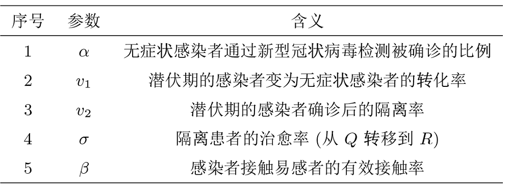
针对 COVID-19 的流行机制, 我们提出一个模型, 该模型考虑 COVID-19 传播的基本特征. 报告的案例中存在确诊患者 (有症状感染者) 和无症状感染者、假阴性患者, 他们都可以感染易感者. 无症状感染者 (asymptomatic patient) 是指无相关临床症状, 核酸检测或血清特异性免疫球蛋白抗体检测阳性者. 假阴性患者则是通过核酸检测或抗体检测等新型冠状病毒检测方法判定为阴性但却感染病毒的个体, 需要多次新型冠状病毒检测才能确诊. 无症状感染者和假阴性患者的临床症状与普通感染者存在较大差异, 但传染率总体上相似. 为方便描述, 将假阴性患者并入无症状感染者一类. 为建立动力学模型, 给出以下假设
(1) 感染者分为有症状与无症状感染者, 他们对易感人群的传染性相同, 这是符合实际情况的. 有关 COVID-19 感染的报告中极少出现无症状感染者自愈的案例, 因此, 忽略少数无症状感染者能够自愈的事实;
(2) COVID-19 的传播途径通常是密切接触传播、呼吸道飞沫传播、气溶胶传播. 本文主要考虑接触传播, 不考虑气溶胶传播, 因此, 假设 COVID-19 的传播方式为密切接触传播和呼吸道飞沫传播 (即易感者仅在接触感染者时才有可能被感染);
(3) 由于 COVID-19 流行的动态比出生和死亡的动态更迅速, 因此, 这里忽略人口动力学因素 (如出生与死亡, 迁入与迁出等);
在人群均匀混合的假设下, 该模型由以下常微分方程组给出
其中, S(t), I(t), A(t), Q(t) 和 R(t) 分别表示 t 时刻健康人群 (易感者), 处于潜伏期的感染者, 无症状感染者, 隔离患者和恢复者数量. 感染新冠后具有一定的潜伏期, 因此, 由易感者 S(t) 被感染后转变的感染者 I(t) 在潜伏期内不会显现感染症状. 随着时间推移, 一部分感染者显现感染症状或者通过核酸检测, 抗体检测等新冠病毒检测方法确诊后被隔离治疗, 成为隔离患者 Q(t), 治愈后移入恢复仓室 R(t); 另一部分感染者不体现感染症状或者经过新型冠状病毒检测无法确诊 (即无症状感染者 A(t)). 经过多次核酸检测或抗体检测等新冠病毒检测方法检测后, 未被确诊的无症状感染者继续参与传播过程; 确诊的无症状感染者则移入隔离仓室退出传播过程.
其中, t=0 为考虑传染病开始传播的时间. 假设初始时刻隔离患者和恢复者的数量为 0 是合理的, 尤其当一种新发传染病入侵某个区域.
图1

由于 ˙S+˙I+˙A+˙Q+˙R=0, 容易得到
且 N0=S0+I0+A0. 注意到, 状态变量 R(t) 不出现在前四个方程中, 我们可以简化系统, 记集合
则不难证明如下结论.
引理 2.1 当 t⩾t0 且初值取在集合 D 中时, 模型 (2.1) 存在唯一的解. 此外, 紧集 D 关于模型 (2.1) 是正向不变的.
该引理表明, 模型 (2.1) 在流行病学和数学角度是有意义的.
3 模型分析
3.1 基本再生数
将模型 (3.1) 在无病平衡点 ε0=(N0,0,0,0,0)T 处线性化, 得到新增感染的出现率和不同仓室间个体的转移率分别为
求上述矩阵在无病平衡点 ε0 处的 Jacobian 矩阵, 得到
通过计算, 易得下一代矩阵为
因此, 模型 (2.1) 的基本再生数为
由基本再生数的表达式可知, 它由两部分构成: (1) 平均潜伏期内一个潜伏期感染者感染的人数, 即 N0βv1+v2; (2) 潜伏期到无症状感染期的比例 v1v1+v2, 乘以未被检测确诊的传染率 N0β(1−α) 和平均确诊时间 1/α.
3.2 最终暴发规模方程
传染病最终暴发规模在数学流行病学中起着重要作用, 是反映传染病暴发严重程度的重要指标之一. 它表示传染病流行结束时, 受到疾病影响的人数, 在种群数量不变的情况下, 传染病暴发规模越大, 疫情越严重, 造成的损失越大, 下面推导模型的最终暴发规模方程. 为分析模型 (2.1) 解的长期行为, 首先给出引理 3.1[14].
引理 3.1 当 t→∞ 时, f(t)→C, 其中, C 为常数, 且存在常数 M⩾0, 对于任意的 t⩾0, 都有 |f″, 则当 t \to + \infty 时, 有 f(t) \to 0.
根据以上引理, 可以得到如下结论.
定理 3.1 对任意的初始值 {S_0} > 0,{I_0} \geqslant 0 和 {A_0} \geqslant 0, 当 t \to + \infty 时, 有 S(t) \to S(\infty ) > 0, I(t) \to 0,A(t) \to 0,Q(t) \to 0,R(t) \to R(\infty ) \geqslant 0, 且 S(\infty ) + R(\infty ) = {N_0}.
证 由模型 (2.1) 的第一个方程可知, \dot S(t) \leqslant 0, 因此 S(t) 是单调非增的, 又因为 S(t) 有下界 0, 当 t \to + \infty 时, S(t) \to S(\infty ). 下证 S(\infty ) > 0, 记 h(l) = - \beta I(l) - \beta (1 - \alpha )A(l), 由模型 (2.1) 的第一个方程可得
进一步可得
都有 S(t) > 0, 故 S(\infty ) > 0. 类似的, 由 \dot R(t) \ge 0且有上界, 可得 R(t) \to R(\infty ) \geqslant 0. 又由于 S(t) + I(t) + A(t) + Q(t) + R(t) \equiv {N_0} , Q(t) \to Q(\infty ) 为常数, 并且 Q'' = \alpha A' + {v_2}I' - \sigma Q' 有界, 因此, 根据引理 3.1, 不难得到 Q(t) \to 0. 类似的, 可以得到 I(t) \to 0, A(t) \to 0, 故 S(\infty ) + R(\infty ) = {N_0}, 结论成立.
当 t \to + \infty 时, 根据定理 3.1 可得, I(\infty ) = A(\infty ) = 0. 考虑下面的简化系统
由系统 (3.3) 的第一个式子, 容易得到
又因为
移项消去 I 前面的系数, 可得
将系统 (3.3) 的第一个式子代入 (3.5) 式中可得
同理可得
将 (3.6) 和 (3.7) 式代入 (3.4) 式, 得到
对 (3.8) 式从 [0,{\text{ + }}\infty ) 积分, 利用 I(\infty ) = A(\infty ) = 0 化简, 得到
结合 R(\infty ) = S(0) + I(0)+ A(0) - S(\infty ) 和 R(\infty ) + S(\infty ) = {N_0}, 可以将上式化简为
因此系统的最终暴发规模隐式方程由 (3.10) 式给出, 进一步, 若初始时刻无症状感染者的数量为 0, 即 A(0)=0, 则 (3.10) 式可以简化为
3.3 隐式方程解的存在唯一性
上一小节得到了最终暴发规模的隐式方程, 下证其隐式方程解的存在唯一性. 令 R(\infty ) = x, 将 (3.11) 式转化为证明存在 {x^ * }, 使得 {x^ * } = f({x^ * }) 成立的不动点问题[17]. 考虑
令
方程 (3.12) 化为f(x) = {N_0} - S(0){{\rm e}^{ - \psi x}}. 对 (3.12) 式分析可以得到下面的结论.
定理 3.2 当 S(0) \in (0,{N_0}) 时, 隐式方程 (3.11) 存在唯一正解 R(\infty ); 当 S(0) = {N_0} 时, 隐式方程存在平凡解 R(\infty ) = 0. 此外, 当 S(0) = {N_0} 且 {R_0} > 1 时, 隐式方程除了平凡解外还有一正解.
证 当 S(0) \in (0,{N_0}) 时, 根据 f(x) 的连续性, 可知
同时, 该函数与 g(x) = x 在区间 (0,{N_0}) 内有交点. 因为该函数从 g(x) = x 图像的上方出发, 穿过 g(x) = x 并到达其下方, 可知解的存在性. 对 f(x) = {N_0} - S(0){{\rm e}^{ - \psi x}} 求二阶导, 可以得到 f''(x) = - S(0){\psi ^2}{{\rm e}^{ - \psi x}} < 0, 故 f(x) 为凹函数, 其图像只与 g(x) = x 交于一点, 故存在唯一一点 {x^*} \in (0,{N_0}), 使得 {x^ * } = f({x^ * }). 因此, 当 S(0) \in (0,{N_0}) 时, 隐式方程 (3.11) 的解存在且唯一. 当 S(0) = {N_0} 时, 由 f(0) = 0 可知, 存在一平凡解 R(\infty ) = 0. 又由于 f(x) 为凹函数, 当 f'(0) < 1 时, 说明函数图像从 g(x) = x 下方开始, 与 g(x) = x 交于唯一一点 x=0; 当 f'(0) >1 时, 说明该函数的图像从 g(x) = x 上方出发, 穿过 g(x) = x 到达其下方, 可以得到另外一个正解, 经计算可得
化简可得
因此, 当 S(0) = {N_0} 且 {R_0} > 1 时, (3.13) 式成立, 同时得到另外一个正解的存在性.
3.4 隐式方程的迭代求解
在 3.3 节中证明了隐式方程解的存在唯一性, 下面通过迭代求隐式方程 (3.11) 的解. 由于方程是不动点形式的, 因此, 设迭代形式为 {x_{n + 1}} = f({x_n}). 为求解方程, 首先给出保证迭代收敛到唯一不动点的一个充分条件, 即引理 3.2[18].
引理 3.2 假设 f 是区间 J 上严格递增的连续函数且具有唯一不动点 {x^ * }, 满足 {x^ * } = f({x^ * }). 另设当 x > {x^ * } 时, x > f(x) 成立; 当 x < {x^ * } 时, x < f(x) 成立, 则从任意的 {x_0} \in J 开始, 迭代序列 {x_{n + 1}} = f({x_n}) 都收敛到不动点 {x^ * }.
应用引理 3.2, 可以得到如下结论.
定理 3.3 当 S(0) \in (0,{N_0}) 或者 S(0) = {N_0} 且 {R_0} \leqslant 1 时, 设 {x^ * } 为函数 f(x) = {N_0} - S(0){{\rm e}^{ - \psi x}} 在区间 [{N_0}] 的不动点; 当 S(0) = {N_0} 且 {R_0} > 1 时, 设 {x^ * } 为 f(x) 的正不动点, 则对于任意的初始值 {x_0} \in (0,{N_0}), 由迭代式 {x_{n + 1}} = f({x_n}) 定义的序列收敛到 {x^ * }.
证 首先考虑最简单的情形, 当S(0) = {N_0} 且 {R_0} \leqslant 1 时, {x^ * } = 0. 由于函数 f(x) 是凹函数, 其图像总是位于 g(x) = x 下方. 因此, 对任意的 x>0 都有 f(x) < x 成立. 即 {x_{n + 1}} = f({x_n}) < {x_n}, 因此, 序列单调递减. 同时, 对于任意的 n, {x_n} 总是非负的, 因此序列 {x_n} 收敛, 其极限则是函数 f(x) 的不动点, 又由于不动点的唯一性, 故序列 {x_n} 收敛到 {x^ * } = 0. 当 {x^ * } > 0 时, 由于 f(x) 为凹函数, 因此, 当 x \in [0,{x^*}) 时, f(x) > x 成立; 当 x \in [{x^*},{N_0}) 时, f(x) < x 成立. 同时, f(x) 的导数为正, 故 f(x) 单调递增. 由引理 3.2 可知, 序列 {x_n} 收敛, 其极限是不动点 {x^ * }. 证毕.
4 传染病的最优控制
自 COVID-19 暴发以来, 人们面临着长期且严峻的挑战, 控制和消灭 COVID-19 成为了当今世界急需解决的一个重大难题. 目前, 人们已提出各种防控措施, 如检疫[19]、隔离[20]、注射疫苗[21]等. 许多地区经过执行严格的防疫政策, 将患病人数、死亡人数降到极低, 但也有些地方仍处于失控状态. 随着时间的推移, 诸多变异菌株开始传播, 它们比常见的菌株传染性更强, 人们感染上变异菌株死亡率更高, 即使通过治疗痊愈, 也可能留下非常严重的后遗症. 因此, 对待 COVID-19 疫情暴发, 有必要采取严格的控制措施. 本节将考虑两组控制策略, 利用 Pontryagin 极值原理来求解两组控制问题, 探究在不同的防疫措施下传染病的流行情况. 第一组控制策略是开展促使易感者采取防疫行为 (即倡导人们采取自我保护行为, 例如戴口罩、保持社交距离和消毒等) 来降低被感染风险的活动 (简称教育活动)[10], 同时, 通过刺激隔离者将自己从隔离状态转移到恢复状态来提高治愈率的活动[21]; 第二组控制策略是开展教育活动和为易感者接种疫苗.
4.1 最优控制问题 C1
第一组控制策略主要考虑降低传染病的传播风险、提高隔离患者的移出率 (治愈率). 基于这个目的, 我们通过降低 COVID-19 暴发期间的感染率来模拟控制效果. 例如, 在 COVID-19 大流行时, 开展一项旨在通过刺激易感者采取保护行为来降低感染率的活动, 以避免被感染病毒. 该措施的实施将会降低易感人群感染病毒的可能性, 同时也会降低因接触无症状感染者而被感染的可能性. 其次, 由于传染性疾病暴发的不可预期性, 医疗资源往往会面临巨大挑战. 感染者数量的激增会导致医疗资源紧缺甚至击穿医疗体系, 故刺激感染者将自己从隔离状态转移到恢复状态也是十分必要的. 因此, 我们同时提高控制期间的治愈率来模拟控制效果.
通过以上说明, 模型 (2.1) 的第一组最优控制问题如下
控制函数 {{u_1}(t)} 和 {{u_2}(t)} 是有界的勒贝格可积函数, {u_1}(t) \in [0.95] 代表教育活动效率, 通过控制 COVID-19 暴发期间的感染率来达到控制疾病的目的; {u_2}(t) \in [\sigma,{\sigma _{\max }}] 为隔离者的恢复率, 当提高恢复率 {{u_2}(t)} 时, 说明更多隔离者恢复, 隔离人数减少, 医疗资源得到缓解. 由于总人口数量保持不变, 因此, 仅考虑 (4.1) 式的前 4 个方程. 此外, 若开展以上措施控制传染病, 实际中则需要付出一定的经济成本, 即 {{u_1}(t)} 和 {{u_2}(t)} 的值越接近上限, 付出成本越高.
理想的控制策略应该具有以下特征: (1) 以较小的最终暴发规模为目标; (2) 以无病平衡点为目标, 通过控制使得系统接近无病平衡点, 使得染病人数清零; (3) 控制在尽可能长的时间内保持较低的成本. 根据以上特征, 定义最小化性能泛函如下
为方便说明, 称以上控制问题为 C1. 我们假设控制成本是非线性二次型的, 考虑到性能泛函三个部分的大小和重要性, 加入系数 {B_1} 和 {B_2} 作为平衡成本. 求解控制问题 C1 需要找到其最优控制 {u_1}^ * 和 {u_2}^ * , 也即
其中, \Omega = \{ ({u_1},{u_2}) \in {L^1}(0,T)|0 \leqslant {u_i} \leqslant 1,i = 1,2\} . 仍在不变集中考虑系统 (4.1), 下面采用 Filippov-Cesari 存在性定理证明最优控制 ({u_1}^ *,{u_2}^ * ) 的存在性, 可以得到下面的结论.
定理 4.1 最优控制问题 C1 的解存在.
证 按照 Filippov-Cesari 存在性定理定义如下集合
其中, X = (S,I,A,Q) 表示状态变量, g(X,{u_1},{u_2}) 表示性能泛函的被积函数, 对任意的 (t,X) \in {R^5}, f(X,{u_1},{u_2}) 为最优控制系统 (4.1) 的右端项. 更确切地说,
下证 Q(t,X) 对每一个 (t,X) 都是凸的, 即任取 {y_1}, {y_2} \in Q(t,X), 存在 \eta \in [0,1], 都有
事实上, 由 {y_1}, {y_2} \in Q(t,X) 可知存在 {\xi _1},{\xi _2} \le 0, {u_{i1}}(t),{u_{i2}}(t),{u_{j1}}(t),{u_{j2}}(t) \in \Omega , 使得
于是, 根据 {y_n} 的第一个分量可得
令 \eta \frac{{{B_1}}}{2}{u_{i1}}^2 + (1 - \eta )\frac{{{B_2}}}{2}{u_{j2}}^2 = {u_3},\eta \frac{{{B_2}}}{2}{u_{i2}}^2 + (1 - \eta )\frac{{{B_1}}}{2}{u_{j1}}^2 = {u_4}. 显然, 有{u_3},{u_4} \in \Omega . 又因为 \eta {\xi _1} + (1 - \eta ){\xi _2} = {\xi _3} \le 0, 说明 {y_n} 的第一个分量属于 Q(t,X).
类似地, 可验证 {y_n} 的第二个分量 \eta f(X,{u_{i1}},{u_{i2}}) + (1 - \eta )f(X,{u_{j1}},{u_{j2}}) 也属于 Q(t,X). 由上可知, {y_n} 的 2 个分量都属于 Q(t,X), 因此, Q(t,X) 是凸的. 显然, \Omega 是一个紧集, 且 X = (S,I,A,Q) 有界, 根据 Filippov-Cesari 存在性定理可知, 结论成立.
最优控制问题 (4.1) 和 (4.2) 的解满足的最优性条件可通过 Pontryagin 极值原理 (PMP) 得到. 根据极值原理, 可以得到下面的定理.
定理 4.2 最优控制问题 C1 存在最优控制 u_1^*(t),u_2^*(t) 和对应的解 {{S^*},{I^*},{A^*},{Q^*}}, 使得极小值 J(u_1^*,u_2^*) \in \Omega , 且存在伴随函数 {\lambda _i}\ (i = 1,\cdots,4), 满足如下方程组
此外, 最优控制 u_1^*,u_2^* 由下式表示
证 根据极值原理, 定义控制问题的哈密顿泛函为
将哈密顿泛函关于状态变量 S,I,A 和 Q 求偏导并在对应的解处取值, 得到伴随函数
因为目标泛函在最终时刻与状态无关, 因此横截条件为零, 即 {\lambda _i}(T) = 0,i = 1,\cdots,4. 根据 Pontryagin 极值原理, 最优控制问题解的表达式通过求解 \partial H / \partial u_{i}=0 \ \ \ (i=1,2) 得到, 求解化简可得
结合控制的上下限, 最优控制被表征为
4.2 最优控制问题 C2
第二组控制策略主要考虑教育活动和易感者接种疫苗相结合的控制策略, 教育活动则是 C1 中所描述的. 从长远看, COVID-19 疫情反反复复. 由于人口流通、贸易往来, 不可避免存在疫情传播, 而 C1 中的控制措施无法长期有效的控制和消灭疫情, 所以接种疫苗格外重要. 现在许多地区正在鼓励易感人群接种疫苗, 但随着病毒的变异, 已接种疫苗的预防能力逐渐降低, 还需要为人们接种最新的疫苗, 降低被感染的风险. 通过以上说明, 模型 (2.1) 的第二组最优控制问题如下
方便起见, 称该问题为 C2, 与最优控制问题 C1 相似, 控制函数 {{u_1}(t)} 和 {{u_2}(t)} 是有界的勒贝格可积函数. {{u_1}(t)} 代表教育活动效率, 通过降低 COVID-19 暴发期间的感染率来达到控制疾病的目的; {{u_2}(t)} 是有效接种率, 假设在控制时间内接种的疫苗完全有效. 当提高有效接种率 {{u_2}(t)} 时, 易感者移入恢复仓室的速率增加, 从而降低易感人数. 类似地, {{u_1}(t)}、{{u_2}(t)} 的值越接近上限, 则控制成本越高. 定义最小化性能泛函如下并记为最优控制问题 C2,
假设控制成本是非线性二次型的, 加入系数 {B_1} 和 {B_2} 作为平衡成本. 与 4.1 节相似, 求解最优控制 C2 需要找到最优控制 {u_1}^ * 和 {u_2}^ * , 也即
其中, \Omega = \{ ({u_1},{u_2}) \in {L^1}(0,T)|0 \le {u_i} \le 1,i = 1,2\} . 同样采用 Filippov-Cesari 存在性定理和 Pontryagin 极值原理证明最优控制 ({u_1}^ *,{u_2}^ * ) 的存在和具体求解, 可以得到下面的定理.
定理 4.3 最优控制问题 C2 的解存在.
定理 4.4 最优控制问题 C2 存在最优控制 u_1^*(t),u_2^*(t) 和对应的解 {{S^*},{I^*},{A^*},{Q^*}}, 使得极小值 J(u_1^*,u_2^*) \in \Omega , 且存在伴随函数 {\lambda _i}\ (i = 1,\cdots,4) 满足如下方程组
此外, 最优控制 u_1^*,u_2^* 由下式给出
定理 4.3 和 4.4 的证明过程类似于定理 4.1 和 4.2, 不再重复说明.
5 数值模拟
在本节中, 我们进行数值模拟以了解最优控制对传染病传播的影响, 并利用迭代法求解最优控制问题 C1 和 C2 的最优控制策略. 为获得模型的参数, 首先对模型进行参数估计.
选取 2020 年 1 月 24 日--2020 年 7 月 28 日浙江省新型冠状病毒感染的数据[22], 主要包括新增病例、累计病例、治愈病例、死亡病例数. 这些病例均经过新型冠状病毒检测, 结果呈阳性. 结合历史累计感染数据, 采用马尔可夫链蒙特卡洛方法[23] (Markov Chain Monte Carlo method) 对模型的参数进行估计, 将 2020 年 1 月 24 日的数据作为初值, 总人口设为 {\text{58}}{\text{.5}} \times {\text{1}}{{\text{0}}^{\text{6}}}. 经估计, 可以得到 \beta {\text{ = 8}}{\text{.83}} \times {\text{1}}{{\text{0}}^{-9}}, \alpha {\text{ = 0}}{\text{.1318}}, {v_1} = 0.00002113, {v_2} = 0.8283, \sigma = 0.1219. 最终暴发规模如图2 所示, 总体拟合效果较好, 以下使用这组参数进行数值模拟.
图2

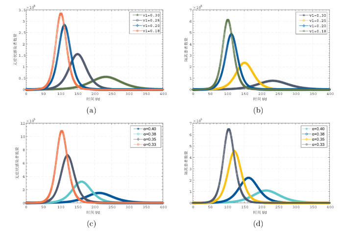
为分析无症状感染者对新冠肺炎传播过程的影响, 图3(a)-(d) 分别展示了 \alpha 、{v_1} 取不同值时模型的演化情形. 图3(a)-(b) 描述了{v_1} 逐渐增大时无症状感染者 A(t) 和隔离患者 Q(t) 的变化情况. 容易发现, 当感染者中无症状感染者的比例出现细微波动时, 无症状感染者的数量将产生巨大变化, 影响新增感染者的数量, 导致需要隔离治疗的患者数量增加, 增加医疗负担. 图3(c)-(d)则展示了 \alpha 取不同值时无症状感染者与隔离患者的数量, 从图3(c)-(d)中容易发现, 当 \alpha 仅从 0.40 减少为 0.38 时, 无症状感染人数便会增加 {\text{2}}{\text{.1438}} 倍. 说明当无症状感染者检测为感染者的比例降低时, 感染数量便会迅速增加, 同时, 隔离人群数量也将激增. 因此, 应增加新冠肺炎检测的频率, 以减少人群中无症状感染者的数量, 降低总的暴发规模.
图3
由于进行卫生教育的成本与教育隔离患者保持健康习惯以至于尽早恢复的成本相似, 因此, 假设第一组控制策略的平衡成本 {{B_1}} 等于{{B_2}}. 借鉴埃塞俄比亚 COVID-19 疫情最优控制问题中选取的平衡成本[24], 选择第一组控制的平衡成本{B_1}={B_2} = 50. 第二组控制进行卫生教育的成本要低于对易感者接种疫苗的成本, 因此, 选择 {B_1} = 50, {B_2} = 150. 图4(a)-(d) 分别绘制了在两组控制下新冠肺炎疫情的传播情况与历史数据的对比. 图4(a) 给出了估计参数下的第一组最优控制, 从图中可发现, 教育活动 {u_1} 需要在控制开始至第 9 天内以最高强度进行, 第 9 天后位于控制下限即可, 控制 {u_2} 可以在控制期限内位于控制下限. 由图4(b) 可知, 最优控制下隔离患者数量的峰值为 148, 峰值时间是 2020 年 1 月 26 日, 相比历史隔离峰值降低了 33.92%. 同时, 隔离曲线的``拉平"速度相比历史数据更加迅速, 说明提高隔离患者的恢复率可以有效降低医疗负担. 截至控制结束, 最终暴发规模为 298 人, 相比不存在控制时降低了 76.54%, 感染人数至 2020 年 2 月 21 日后不再增加. 图4(c) 展示了估计参数下的第二组最优控制, 容易发现, 在第二组控制下, 教育活动 {u_1} 需要在控制开始至第 11 天内以最高强度进行, 11 天后位于控制下限, 疫苗接种则需要在 24-70 天内保持最高接种率. 图4(d) 比较了最优控制下感染者数量与历史数据的对比. 由于许多易感者接种疫苗移入恢复仓室, 不能以最终暴发规模作为考量, 但从图4(d) 中仍能发现, 在第二组最优控制下感染者数量在 1月 29 日后便趋向于 0. 控制结果说明在面对新冠肺炎或其他新发传染病的传播时, 降低传染率和为易感者接种疫苗是控制疫情发展的有效手段, 提高隔离患者的恢复率是有效降低医疗负担的手段.
图4
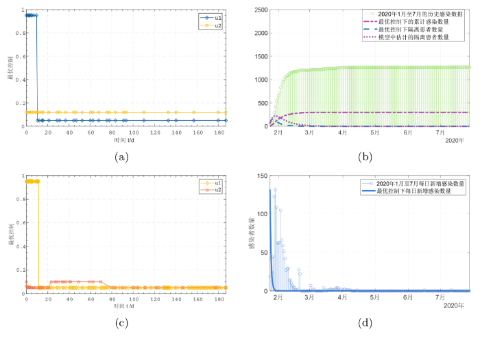
图4
模型的最优控制与最优控制下模型结果同感染数据对比, 图(a)-(b) 中 {B_1}={B_2} = 50, 图(c)-(d) 中 {B_1}=50, {B_2} = 150, 其余参数皆与参数估计结果保持一致, 控制持续时间为 187 天.
6 讨论
本文以新冠病毒 (COVID-19) 的群体传播为背景, 提出了一个具有无症状感染和隔离的 SIAQR 模型, 讨论了模型的基本特性, 研究了模型的基本再生数、最终暴发规模, 以及最终暴发规模隐式方程解的存在唯一性与可解性. 在此基础上, 为控制疫情传播, 考虑了两种可能的控制策略, 采用 Filippov-Cesari 存在性定理和 Pontryagin 极值原理分析最优控制问题解的存在性. 为了对模型参数进行估计, 选取浙江省新冠肺炎感染的历史数据采用马尔可夫链蒙特卡洛方法对模型参数进行了估计. 根据估计的参数进行数值模拟, 对比了不同参数对疫情传播的影响和最优控制对新冠病毒传播行为的影响. 结果说明, 当感染者中无症状感染者的比例增大时, 应对人群增加对应的新型冠状病毒检测. 同时, 在估计参数下, 最优控制可以降低 33.92% 的隔离患者峰值、76.54% 的最终暴发规模, 能够有效控制疫情传播. 因此, 面对新冠肺炎或者新发传染病的传播, 降低传染率和为易感者接种疫苗仍是控制疫情发展或者降低医疗负担的有效手段.
在我们的模型中, 忽略了直接恢复的感染者, 但事实已经证明, 感染者和无症状感染者都有可能直接恢复, 同时, 感染新冠肺炎后存在一定的潜伏期, 若在模型中考虑直接恢复和潜伏期等因素,这样得到的模型更加全面合理[25]. 其次, 现实世界中传染病的传播会受到许多外部随机因素的影响, 如温度、湿度等, 通常会影响人口动力学和模型的动力学动态, 因此, 具有随机扰动的传染病模型可以更准确的描述随机因素对传染病传播的影响[26]. 若引入随机扰动, 我们的模型可以扩展成随机传染病模型, 或许可以得到更符合真实数据的数值结果. 最后, Cadoni[27]通过 I(S) = {I_0} + ({S_0} - S) + \frac{\beta }{\alpha }\log (\frac{S}{{{S_0}}}) 来刻画 Susceptible-Infectious-Recovered (SIR) 模型中感染者的峰值, 从而确定如何减少疫情高峰及峰值. 若可以类似地获得一个刻画 SIAQR 模型中峰值到达时间和感染峰值的显式或隐式方程, 结合最优控制理论或动态规划等方法, 我们的模型可以进一步用于分析如何控制感染峰值或降低最终暴发规模问题. 为降低医疗负担, 也可以考虑将目标函数设为隔离患者的高峰值, 这些问题我们留待进一步探索, 降低感染者高峰也需要进一步研究.
参考文献
跟踪严重急性呼吸综合症冠状病毒 2 变异株
https://www.who.int/zh/activities/tracking-SARS-CoV-2-variants [2022-4-14]
2019 冠状病毒病 (COVID-19) 疫情
https://www.who.int/zh/emergencies/diseases/novel-coronavirus-2019 [2022-4-14]
Assessing age-specific vaccination strategies and post-vaccination reopening policies for COVID-19 control using SEIR modeling approach
DOI:10.1007/s11538-022-01064-w
PMID:36029391
[本文引用: 1]

As the availability of COVID-19 vaccines, it is badly needed to develop vaccination guidelines to prioritize the vaccination delivery in order to effectively stop COVID-19 epidemic and minimize the loss. We evaluated the effect of age-specific vaccination strategies on the number of infections and deaths using an SEIR model, considering the age structure and social contact patterns for different age groups for each of different countries. In general, the vaccination priority should be given to those younger people who are active in social contacts to minimize the number of infections, while the vaccination priority should be given to the elderly to minimize the number of deaths. But this principle may not always apply when the interaction of age structure and age-specific social contact patterns is complicated. Partially reopening schools, workplaces or households, the vaccination priority may need to be adjusted accordingly. Prematurely reopening social contacts could initiate a new outbreak or even a new pandemic out of control if the vaccination rate and the detection rate are not high enough. Our result suggests that it requires at least nine months of vaccination (with a high vaccination rate > 0.1%) for Italy and India before fully reopening social contacts in order to avoid a new pandemic.© 2022. The Author(s), under exclusive licence to Society for Mathematical Biology.
Estimation of the transmission risk of the 2019-nCoV and its implication for public health interventions
DOI:10.3390/jcm9020462
URL
[本文引用: 1]
Since the emergence of the first cases in Wuhan, China, the novel coronavirus (2019-nCoV) infection has been quickly spreading out to other provinces and neighboring countries. Estimation of the basic reproduction number by means of mathematical modeling can be helpful for determining the potential and severity of an outbreak and providing critical information for identifying the type of disease interventions and intensity. A deterministic compartmental model was devised based on the clinical progression of the disease, epidemiological status of the individuals, and intervention measures. The estimations based on likelihood and model analysis show that the control reproduction number may be as high as 6.47 (95% CI 5.71–7.23). Sensitivity analyses show that interventions, such as intensive contact tracing followed by quarantine and isolation, can effectively reduce the control reproduction number and transmission risk, with the effect of travel restriction adopted by Wuhan on 2019-nCoV infection in Beijing being almost equivalent to increasing quarantine by a 100 thousand baseline value. It is essential to assess how the expensive, resource-intensive measures implemented by the Chinese authorities can contribute to the prevention and control of the 2019-nCoV infection, and how long they should be maintained. Under the most restrictive measures, the outbreak is expected to peak within two weeks (since 23 January 2020) with a significant low peak value. With travel restriction (no imported exposed individuals to Beijing), the number of infected individuals in seven days will decrease by 91.14% in Beijing, compared with the scenario of no travel restriction.
Control of COVID-19 dynamics through a fractional-order model
DOI:10.1016/j.aej.2021.02.022 URL [本文引用: 1]
Predicting the cumulative number of cases for the COVID-19 epidemic in China from early data
DOI:10.3934/mbe.2020172
PMID:32987515
[本文引用: 1]
We model the COVID-19 coronavirus epidemic in China. We use early reported case data to predict the cumulative number of reported cases to a final size. The key features of our model are the timing of implementation of major public policies restricting social movement, the identification and isolation of unreported cases, and the impact of asymptomatic infectious cases.
Predicting the number of reported and unreported cases for the COVID-19 epidemics in China, South Korea, Italy, France, Germany and United Kingdom
DOI:10.1016/j.jtbi.2020.110501 URL [本文引用: 1]
Optimal control of aquatic diseases: A case study of Yemen's cholera outbreak
DOI:10.1007/s10957-020-01668-z [本文引用: 1]
Controlling propagation of epidemics via mean-field control
DOI:10.1137/20M1342690 URL [本文引用: 1]
Optimal control of an epidemic through educational campaigns
新型冠状病毒肺炎疫情控制策略研究:效率评估及建议
Study on the control strategy of novel coronavirus pneumonia outbreak: Efficiency assessment and recommendations
Reproduction numbers and sub-threshold endemic equilibria for compartmental models of disease transmission
DOI:10.1016/S0025-5564(02)00108-6 URL [本文引用: 1]
On the definition and the computation of the basic reproduction ratio {R_0} in models for infectious diseases in heterogeneous populations
DOI:10.1007/BF00178324
PMID:2117040
[本文引用: 1]
The expected number of secondary cases produced by a typical infected individual during its entire period of infectiousness in a completely susceptible population is mathematically defined as the dominant eigenvalue of a positive linear operator. It is shown that in certain special cases one can easily compute or estimate this eigenvalue. Several examples involving various structuring variables like age, sexual disposition and activity are presented.
Epidemic dynamics of influenza-like diseases spreading in complex networks
DOI:10.1007/s11071-020-05867-1 [本文引用: 1]
Solvability of implicit final size equations for SIR epidemic models
DOI:10.1016/j.mbs.2016.10.012 URL [本文引用: 1]
Resource allocation for control of infectious diseases in multiple independent populations: Beyond cost-effectiveness analysis
Traditional cost-effectiveness analysis (CEA) assumes that program costs and benefits scale linearly with investment-an unrealistic assumption for epidemic control programs. This paper combines epidemic modeling with optimization techniques to determine the optimal allocation of a limited resource for epidemic control among multiple noninteracting populations. We show that the optimal resource allocation depends on many factors including the size of each population, the state of the epidemic in each population before resources are allocated (e.g. infection prevalence and incidence), the length of the time horizon, and prevention program characteristics. We establish conditions that characterize the optimal solution in certain cases.
Modeling the role of information and limited optimal treatment on disease prevalence
DOI:S0022-5193(16)30382-4
PMID:27890574
[本文引用: 2]
Disease outbreaks induce behavioural changes in healthy individuals to avoid contracting infection. We first propose a compartmental model which accounts for the effect of individual's behavioural response due to information of the disease prevalence. It is assumed that the information is growing as a function of infective population density that saturates at higher density of infective population and depends on active educational and social programmes. Model analysis has been performed and the global stability of equilibrium points is established. Further, choosing the treatment (a pharmaceutical intervention) and the effect of information (a non-pharmaceutical intervention) as controls, an optimal control problem is formulated to minimize the cost and disease fatality. In the cost functional, the nonlinear effect of controls is accounted. Analytical characterization of optimal control paths is done with the help of Pontryagin's Maximum Principle. Numerical findings suggest that if only control via information is used, it is effective and economical for early phase of disease spread whereas treatment works well for long term control except for initial phase. Furthermore, we observe that the effect of information induced behavioural response plays a crucial role in the absence of pharmaceutical control. Moreover, comprehensive use of both the control interventions is more effective than any single applied control policy and it reduces the number of infective individuals and minimizes the economic cost generated from disease burden and applied controls. Thus, the combined effect of both the control policies is found more economical during the entire epidemic period whereas the implementation of a single policy is not found economically viable.Copyright © 2016 Elsevier Ltd. All rights reserved.
An introduction to MCMC for machine learning
DOI:10.1023/A:1020281327116 URL [本文引用: 1]
Mathematical modeling and optimal control analysis of COVID-19 in Ethiopia
DOI:10.1080/09720502.2021.1874086 URL [本文引用: 1]
Stability and extinction of SEIR epidemic models with generalized nonlinear incidence
DOI:10.1016/j.matcom.2018.09.029 URL [本文引用: 1]
Stationary distribution and density function of a stochastic SVIR epidemic model
DOI:10.1016/j.jfranklin.2022.09.026 URL [本文引用: 1]
How to reduce epidemic peaks keeping under control the time-span of the epidemic
DOI:10.1016/j.chaos.2020.109940 URL [本文引用: 1]
