

1 引言
近年来, 为实现公司价值最大化而控制分红以及风险暴露的风险模型引起了很多学者的关注.
如在指数保费准则下的最优策略[5], 带终值的问题[17], 保险人和再保险人采取两类保费原则的问题[13], 流动性价值约束的问题[20]. 同时, 保险监管机构必须注意构建偿付能力监管体系, 如巴塞尔协议II和巴塞尔协议 III. 因此, 最近对受偿付能力约束的优化问题的研究越来越多. 如文献 [4,8,10,11,12], 在这些文献中, 偿付能力约束主要集中在盈余过程或政策上. 另一方面, 保险公司的管理者必须考虑监管机构的随机偿付能力监管时间, 并希望在监管时间做出更好的表现. 在人寿保险公司中, 文献 [6] 表明监管制度应迫使保险公司在困境中降低资产配置的风险性. 在一个基于效用的框架中, 引入这样一个系统可以增加投保人的利益, 而不会恶化保险公司的利益. 同时, 违约概率 (以及由此产生的偿付能力资本要求) 可以降低. 与文献 [6] 类似, 大多数研究集中于随机寿命对个人决策的影响, 很少有论文研究公司的情况, 这促使我们考虑具有这种随机时间的分红支付. 在数学上, 本文讨论的问题被表述为随机时间区间的最优分红. 对于经典风险模型, 最先的工作可以参考文献 [1]. 后续的工作有文献 [22] 研究了对偶风险模型.
本文的工作可以概括为以下几点. 我们在模型中引入了随机时间和品牌价值, 这个模型是有实际意义的. 通过求解与该控制问题相关的 HJB 方程, 我们得到了明确的最优策略和值函数. 本文的结构安排如下: 第 2 节介绍了本文的模型框架, 以及与该控制问题相关的 HJB 方程和值函数的估计. 第 3 节给出了求解 HJB 方程和最优策略的详细过程. 结果显示, 根据品牌价值的范围, 最优的分红和再保险策略以及最大的公司价值表现出三种不同的形式. 第 4 节介绍了一个数值例子.
2 问题的描述和值函数的估计
设 (Ω, F, Ft,P) 是一个完备的概率空间, 包含本文中所有的随机过程和随机变量. 假设无控制情况下的盈余过程为
初始盈余为 X(0)=x≥0, 其中 μ,σ>0, {W(t)}t≥0 是标准布朗运动. 保险人向股东支付分红并通过比例再保险控制风险. 设在时刻 t, aπ(t) 为保险人自留的风险比例, 1−aπ(t) 为向再保险人转移的比例. Lπ(t) 为到时刻 t 支付的分红总额. 本文假设再保险是便宜的, 即再保险的相对安全负载和原保险相同. 为继续我们的讨论, 首先给出容许控制策略的定义.
定义 2.1(容许控制策略) 一个控制策略 π 是一个二维随机过程 {aπ(t),Lπ(t)}t≥0, 如果它适应于 Ft 且满足
(1) aπ(t)∈[0,1],
(2) Lπ(t) 是非负, 非降, 且右连左极的,
(3) dLπ(t)≤Xπ(t−), 其中 Xπ(t−) 由下面的 (2.2) 式给出.
则称之为容许控制策略.
定义 Π 为所有容许控制策略的集合. 与文献 [9] 一样, 在便宜再保险和策略 π={aπ(t),Lπ(t)}t≥0 下的盈余过程为
根据文献 [1] 中思想, 记随机到达时间为 τ, 服从均值为 1λ 的指数分布, 且独立于盈余过程 {Xπ(t)}t≥0. 令 τπ=inf ( \inf\{\varnothing\}=\infty ) 表示控制策略 \pi 下的破产时间. 如引言中介绍的那样, 该机制的运行情况如下: 若 \tau_\pi>\tau , 保险人在 \tau 时刻得到 X_\pi(\tau)+P ; 若 \tau_\pi<\tau , 保险人在时刻 \tau_\pi 得到品牌价值 P . 对给定策略 \pi\in\Pi , 定义性能函数 J_{\pi}(x) 为
其中 \mathbb{E}_{x}[\cdot]=\mathbb{E}[\cdot|X(0)=x] , \delta>0 为折现率, I_{A} 为集合 A 上的示性函数. 可将 J_{\pi}(x) 重新表示成如下形式
定义值函数 V(x) 为 \Pi 上最优的性能函数, 即
一个策略 \pi^{*}\in\Pi 称为最优的, 若 V(x)=J_{\pi^{*}}(x) . 本文的目的就是找到最优策略和值函数.
对任意 a\in[0,1] , 定义微分算子 \mathscr{A}_{a}g(x) 为
其中 g(\cdot) 是光滑函数.
若值函数是光滑的, 即 V(x)\in C^{2}(0, \infty) , 则由动态规划原理知, V(x) 满足 Hamilton-Jacobi-Bellman (HJB) 方程
和边界条件
下面的定理 2.1 表明, 满足 HJB 方程 (2.6) 和 (2.7) 的解不小于值函数, 这使我们能够通过求解HJB 方程得到值函数.
定理 2.1 若函数 f(x)\in C^{2}[0, \infty) 是递增的, 凹的, 且满足条件: f(0)=P 和 \max \{1-f'(x), \sup\limits_{a\in[0,1]}\mathscr{A}_{a}f(x)\}\leq0 , 则 f(x)\geq V(x), x\in[0, \infty) .
证 对任意 \pi\in\Pi . 记 \mathscr{T}=\{s:L_{\pi}(s-)\neq L_{\pi}(s)\} . 令 \widetilde{L}_{\pi}(t)=\sum\limits_{s\in\mathscr{T}, s\leq t}(L_{\pi}(s)-L_{\pi}(s-)) 为 L_{\pi}(t) 的不连续部分, \overline{L}_{\pi}(t)=L_{\pi}(t)-\widetilde{L}_{\pi}(t) 为 L_{\pi}(t) 的连续部分. 对 0<\varepsilon<x , 定义 \tau_{\pi, \varepsilon}=\inf\{t:X_{\pi}(t)\leq \varepsilon\} . 由广义伊藤公式知
因为 f(x) 是凹函数, 所以 f'(x) 递减且在 (0, t\wedge\tau_{\pi, \varepsilon}] 上 f'(x)\leq f'(\varepsilon) , 从而有
由 f'(x)\geq 1 知, f(X_{\pi}(s))-f(X_{\pi}(s-))\leq -[L_{\pi}(s)-L_{\pi}(s-)] . 对 (2.8) 式两边取期望有
由 f(x) 的凹性知, f(x)\leq \alpha x+\beta 对某 \alpha, \beta>0 成立. 因此
其中常数 \gamma>0 不依赖于 \varepsilon . 进而
在 (2.9) 式中令 t\rightarrow\infty , 有
在 (2.10) 式中令 \varepsilon\rightarrow 0 , 因为 \tau_{\pi, \varepsilon}\uparrow\tau_{\pi} , 由控制收敛定理知 f(x)\geq J_{\pi}(x) . 由 \pi 的任意性知 f(x)\geq V(x) .
3 值函数和最优策略的表达式
本节我们将努力寻找满足 (2.6) 式和边界条件 (2.7) 的一个递增的且二阶连续可微的凹解 f(x) . 令 x_0=\sup\{x:f'(x)>1, x\geq 0\} . 若 x_{0}>0 , 则有
购买再保险的目的是避免破产, 所以我们猜想最优再保险策略为: 当盈余低于 x_1 时, 购买部分再保险; 当盈余不低于 x_1 时, 不购买再保险. 最优化问题将根据 x_0 和 x_1 的值分为三种情形.
情形 1 x_0=0
在该情形下, f(x)=x+P , 这是一个性能函数, 相应的策略为: 将所有的盈余作为分红支付, 破产立即发生. 为了确保 f(x)=x+P 是 (2.6) 和 (2.7) 式的解, 我们需要条件 \mathscr{A}_{a}f(x)\leq0 , 这等价于 P\geq \frac{\mu}{\delta} . 由定理 2.1, 我们有 f(x)=V(x) . 我们将这个结果总结为下面的定理 3.1.
定理 3.1 若 P\geq \frac{\mu}{\delta} , 则 V(x)=x+P , 相应的策略为: 将所有的盈余作为分红支付.
情形 2 x_0>0 , x_1=\infty
在该情形下, 当 x\geq x_0 时,
当 0<x<x_0 时,
(3.3) 式的解具有形式
其中 A_1, \ A_2 为常数, r_{1, 2}=\frac{-\mu\pm\sqrt{\mu^{2}+2\sigma^{2}(\lambda+\delta)}}{\sigma^{2}} 是特征方程 \frac{\sigma^{2}}{2}r^{2}+\mu r-(\lambda+\delta)=0 的两个根. 由初始条件 f(0)=0 得
使用光滑契合的方法, 我们有 f'(x_0+)=f'(x_0-)=1 和 f''(x_0+)=f''(x_0-)=0 , 即
和
由 (3.6) 和 (3.7) 式得
和
将 (3.8) 和 (3.9) 式代入 (3.5) 式, 可得
x_0 可由 (3.10) 式确定. 下面引理给出 (3.10) 式有唯一正数解 x_0 的条件.
引理 3.1 若 P<\frac{\mu}{\delta} , 则 (3.10) 式有唯一正数解 x_0 .
证 令 R_1(x)=-\frac{r_2}{r_1(r_1-r_2)}{\rm e}^{-r_1x}+\frac{r_1}{r_2(r_1-r_2)}{\rm e}^{-r_2x} , 则 R_1(\infty)=-\infty 且 R_1'(x)=\frac{r_2}{r_1-r_2}{\rm e}^{-r_1x}-\frac{r_1}{r_1-r_2}{\rm e}^{-r_2x}<0 . 我们仅需证明 R_1(0)=\frac{r_1+r_2}{r_1r_2}=\frac{\mu}{\lambda+\delta}>P-\frac{\lambda\mu}{\delta(\lambda+\delta)} , 这在条件 P<\frac{\mu}{\delta} 下是显然的.
令 R_2(x)=\frac{r_1(r_1-r_2)}{r_1+r_2}x+\frac{\lambda}{\delta}+\big{[}\frac{r_2(r_1-r_2)}{r_1+r_2}x-\frac{\lambda}{\delta}\big{]}^{\frac{r_1}{r_2}} . 因为 R_2(x) 是减函数, R_2(x)\rightarrow\infty ( x\rightarrow \frac{\lambda(r_1+r_2)}{\delta r_2(r_1-r_2)}+ ) 和 R_2\big{(}\frac{\mu}{\delta}\big{)}<-\frac{\mu r_1r_2}{\delta(r_1+r_2)}+\frac{\lambda}{\delta}+\big{[}\frac{\mu r_1r_2}{\delta(r_1+r_2)}-\frac{\lambda}{\delta}\big{]}^{\frac{r_1}{r_2}}=0 可知 R_2(x)=0 有唯一解 P_{0}\in\big{(}\frac{\lambda(r_1+r_2)}{\delta r_2(r_1-r_2)}, \frac{\mu}{\delta}\big{)} .
定理 3.2 若 P_0<P<\frac{\mu}{\delta} , 则
是 (2.6) 和 (2.7) 式的一个递增且二阶连续可微的凹解, 其中 x_0 由 (3.10) 式确定.
证 显然 f(x) 是一个递增且二阶连续可微的凹函数. 对 x\geq x_0 , 1-f'(x)=0 且
对 x< x_0 , 由 f(x) 的凹性知 1-f'(x)<0 . 由 f(x) 的构造知, 当 a=1 时, \mathscr{A}_{a}f(x)=0 , 我们仅需表明 (2.6) 式在 a=1 达到上确界, 这等价于证明 -\frac{\mu f'(x)}{\sigma^{2}f''(x)}> 1 对 x< x_0 成立.
因为 P>P_0 , 且 R_2(x) 是一个减函数, R_2(P)<R_2(P_0)=0 , 所以
且有 R_1(x_0)=P-\frac{\lambda\mu}{\delta(\lambda+\delta)}>R_1(-\frac{\text{log}(\frac{Pr_2(r_1-r_2)}{r_1+r_2}-\frac{\lambda}{\delta})}{r_2}). 因为 R_1(x) 是一个减函数, 所以 x_0<-\frac{\text{log}(\frac{Pr_2(r_1-r_2)}{r_1+r_2}-\frac{\lambda}{\delta})}{r_2}, 从而
由 (3.10) 式知
令 R_3(x)=\frac{\delta}{r_1-r_2}[2(\lambda+\delta)-\mu r_2]{\rm e}^{r_1(x-x_0)}-\frac{\delta}{r_1-r_2}[2(\lambda+\delta)-\mu r_1]{\rm e}^{r_2(x-x_0)}+\lambda\mu . 注意到 2(\lambda+\delta)-\mu r_1>0 , 我们知道 R_3(x) 是一个增函数. 使用 \frac{r_1+r_2}{r_1r_2}=\frac{\mu}{\lambda+\delta} , 我们得到
因此对 x<x_0 ,
从而 -\frac{\mu f'(x)}{\sigma^{2}f''(x)}> 1 .
情形 3 0<x_1<x_0<\infty
在该情形下, 对 0<x<x_1 , (2.6) 的上确界在 a=-\frac{\mu f'(x)}{\sigma^{2}f''(x)} 达到, 因此有
对 x_1<x<x_0 ,
对 x\geq x_0 ,
(3.13) 式的解具有形式
其中 C_1, \ C_2 为常数, r_1, \ r_2 和情形2相同. 使用光滑契合的方法, 我们有 f'(x_0+)=f'(x_0-)=1 和 f''(x_0+)=f''(x_0-)=0 , 即
从而有
和
使用文献 [9] 中的方法, 存在函数 h:\ R\rightarrow [\infty] , 使得
因此
由 (3.19) 式知 h(z) 是一个增函数. 在 (3.12) 式中令 x=h(z) 并使用 (3.18) 和 (3.19) 式, 有
对 (3.20) 式两边关于 z 求导可得
其中 m=\frac{2\sigma^{2}\lambda}{\mu^{2}}, \ n=\frac{\mu^{2}+2\sigma^{2}(\lambda+\delta)}{\mu^{2}} . (3.21) 式的一般解具有形式
其中 B_1, \ B_2 为常数. 由 (3.18) 式和初值条件 f(0)=P , 有
将 (3.23) 式代入 (3.12) 式并令 x 趋向于 0 有
由 h(h^{-1}(0))=0 知
将 (3.25) 式代入 (3.22) 式并使用 (3.24) 式, 有
使用光滑契合的方法, 有 f'(x_1+)=f'(x_1-) , f''(x_1+)=f''(x_1-) 和 \frac{\mu f'(x_1)}{\sigma^{2}f''(x_1)}=1 , 即
和
定义 x_{*}=x_1-x_0 并令 R_4(x)=\delta r_2{\rm e}^{r_1x}+\delta r_1{\rm e}^{r_2x}+\lambda(r_1+r_2) . 因为 R_4(x) 是一个减函数, R(0)=(\lambda+\delta)(r_1+r_2)<0 和 R(-\infty)=+\infty , 可知 x_{*} 存在且 x_{*}<0 . 由 (3.27) 式知
由 (3.28) 和 (3.30) 式知
h^{-1}(0) 可由 (3.31) 式确定.
引理 3.2 若 0<P\leq P_0 , 则 h^{-1}(0)<0 .
证 若 \frac{Pr_2(r_1-r_2)}{r_1+r_2}-\frac{\lambda}{\delta}<1 , 则 {\rm e}^{r_2x_{*}}>1>\frac{Pr_2(r_1-r_2)}{r_1+r_2}-\frac{\lambda}{\delta} . 若 \frac{Pr_2(r_1-r_2)}{r_1+r_2}-\frac{\lambda}{\delta}\geq1 , 因为 P\leq P_0 , 我们有 R_2(P)\geq R_2(P_0)=0 , 因此
这等价于 R_4({\frac{1}{r_2}}\text{log}\big{[}\frac{Pr_2(r_1-r_2)}{r_1+r_2}-\frac{\lambda}{\delta}\big{]})\leq 0=R_4(x_{*}) , 因此 {\rm e}^{r_2x_{*}}>\frac{Pr_2(r_1-r_2)}{r_1+r_2}-\frac{\lambda}{\delta} , 则
(3.29) 和 (3.30) 式表明
(3.29), (3.31) 和 (3.33) 式表明
(3.32)-(3.34) 式表明
令 R_5(x)={\rm e}^{(n-1)x-m{\rm e}^{x}} . 因为当 x\leq 0 时,
所以 R_5(x) 在 (-\infty, 0] 上是一个增函数. 由 (3.35) 式知 h^{-1}(0)<-\text{log}(u_{*})<0 .
注 3.1 由 (3.30) 式知 h^{-1}(x_1)=-\text{log}(u_{*})>h^{-1}(0) . 因为 h^{-1}(x) 是一个增函数, 所以 x_1>0 .
定理 3.3 若 0<P\leq P_0 , 则
是 (2.6) 和 (2.7) 式的一个递增且二阶连续可微的凹解, 其中 h^{-1}(0) 由 (3.31) 式确定, x_1=h(-\log u_*) , x_0=x_1-x_* .
证 和定理 3.2 证明的方法类似, 可以验证 f(x) 是一个递增且二阶连续可微的凹函数, 且当 x>x_1 时, f(x) 满足 (2.6) 和 (2.7) 式. 由 f(x) 的构造知, 当 a=-\frac{\mu f(x)}{\sigma^{2}f''(x)} 时, \mathscr{A}_{a}f(x)=0 , 仅需验证 (2.6) 的上确界在 a=-\frac{\mu f(x)}{\sigma^{2}f''(x)} 达到, 这等价于证明当 x<x_1 时, -\frac{\mu f'(x)}{\sigma^{2}f''(x)}<1 . 记 a(x)=-\frac{\mu f'(x)}{\sigma^{2}f''(x)} . 使用 h(x) 在 (3.22) 式中的表达式, 可得
因为 h(x) 是一个增函数, 所以 [h^{-1}(x)]'>0 且当 x<x_1 时,
由 (3.24) 式知 B_1>0 . 因此当 x<x_1 时,
注意到 a(x_1)=1 , 我们有, 当 x<x_1 时, a(x)<a(x_1)=1 .
下面的定理 3.4 验证在策略 \pi^{*} 下的性能函数就是值函数, 从而 \pi^{*} 是最优策略.
定理 3.4 若 P_0<P<\frac{\mu}{\delta} , 定义 \pi^{*} 为 a_{\pi^{*}}(t)=1 , 分红策略是障碍值为 x_0 的障碍策略, x_0 和 f(x) 由定理 3.2 给出; 若 0<P\leq P_0 , 定义 \pi^{*} 为 a_{\pi^{*}}(t)=-\frac{\mu f'(X_{\pi^{*}}(t))}{\sigma^{2}f''(X_{\pi^{*}}(t))} , x\leq x_1 和 a_{\pi^{*}}(t)=1 , x_1<x<x_0 , 分红策略是障碍值为 x_0 的障碍策略, x_0 和 f(x) 由定理 3.3 给出. 则
证 将 \pi^{*} 代替 (2.8) 式中 \pi , (2.8) 式成为一个等式, 所以有
因为在 \{\tau_{\pi^{*}}<\infty\} 上, 当 \varepsilon\rightarrow 0 时, \tau_{\pi^{*}, \varepsilon}\rightarrow \tau_{\pi^{*}} , X_{\pi^{*}}(\tau_{\pi^{*}})=0 且 f(0)=P , 所以
因为在 \{\tau_{\pi^{*}}=\infty\} 上, 当 \varepsilon\rightarrow 0 时, \tau_{\pi^{*}, \varepsilon}\rightarrow \infty , 所以
在 (3.36) 式中令 \varepsilon\rightarrow 0 , 有
证毕.
4 数值例子
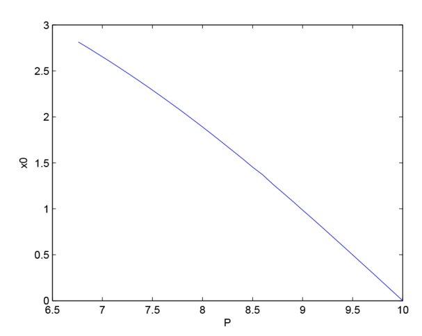
本节将提供一个数值例子. 令 \mu=1, \ \sigma=2, \ \delta=0.1, \ \lambda=0.05 , 可得 P_{0}=6.76 , \frac{\mu}{\delta}=10 .
图1 是最优障碍值 x_0 作为 P 的函数的图像, P\in (P_0, \frac{\mu}{\delta}) . 可以看出 x_0 关于 P 是一个减函数, 且当 P\rightarrow 10 时, x_0\rightarrow 0 , 这与 P=\frac{\mu}{\delta}=10 的情形相符.
图1
若 P=8 , 则 x_0=1.89 , 我们得到值函数
其曲线如图2 所示.
图2
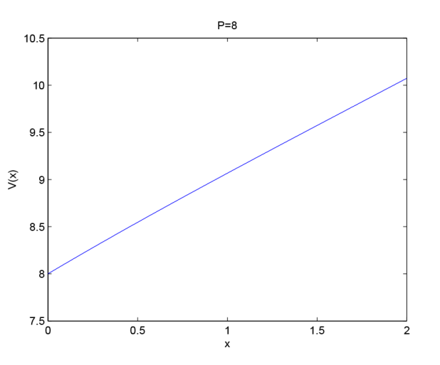
图3

图4
参考文献
Optimal dividend and investment problems under Sparre Andersen model
Optimal dividends in an Ornstein-Uhlenbeck type model with credit and debit interest
DOI:10.1080/10920277.2006.10596250 URL [本文引用: 1]
Optimal asset allocation in life insurance: The impact of regulation
DOI:10.1017/asb.2016.12
URL
[本文引用: 1]

In a typical equity-linked life insurance contract, the insurance company is entitled to a share of return surpluses as compensation for the return guarantee granted to the policyholders. The set of possible contract terms might, however, be restricted by a regulatory default constraint — a fact that can force the two parties to initiate sub-optimal insurance contracts. We show that this effect can be mitigated if regulatory policy is more flexible. We suggest that the regulator implement a traffic light system where companies are forced to reduce the riskiness of their asset allocation in distress. In a utility-based framework, we show that the introduction of such a system can increase the benefits of the policyholder without deteriorating the benefits of the insurance company. At the same time, default probabilities (and thus solvency capital requirements) can be reduced.
Optimal dividend problem with a nonlinear regular-singular stochastic control
DOI:10.1016/j.insmatheco.2013.02.010 URL [本文引用: 1]
Optimal risk and dividend strategies with transaction costs and terminal value
DOI:10.1016/j.econmod.2016.01.009 URL [本文引用: 3]
Controlling risk exposure and dividends payout schemes: Insurance company example
DOI:10.1111/mafi.1999.9.issue-2 URL [本文引用: 2]
Optimal dividend payouts for diffusions with solvency constraints
DOI:10.1007/s007800200098 URL [本文引用: 1]
Optimal dividend and investing control of a insurance company with higher solvency constraints
DOI:10.1016/j.insmatheco.2011.08.008 URL [本文引用: 1]
Optimal dividend-reinsurance with two types of premium principles
DOI:10.1017/S0269964815000352
URL
[本文引用: 1]
A combined optimal dividend/reinsurance problem with two types of insurance claims, namely the expected premium principle and the variance premium principle, is discussed. Dividend payments are considered with both fixed and proportional transaction costs. The objective of an insurer is to determine an optimal dividend–reinsurance policy so as to maximize the expected total value of discounted dividend payments to shareholders up to ruin time. The problem is formulated as an optimal regular-impulse control problem. Closed-form solutions for the value function and optimal dividend–reinsurance strategy are obtained in some particular cases. Finally, some numerical analysis is given to illustrate the effects of safety loading on optimal reinsurance strategy.
Optimal risk and dividend distribution control models for an insurance company
DOI:10.1007/s001860050001 URL [本文引用: 2]
Optimality of barrier dividend strategy in a jump-diffusion risk model with debit interest
DOI:10.1007/s10998-020-00338-x [本文引用: 1]
Optimal reinsurance and dividend strategies under the Markov-modulated insurance risk model
DOI:10.1080/07362994.2010.515488 URL [本文引用: 1]
Optimal risk control and dividend distribution policies for a diffusion model with terminal value
DOI:10.1016/j.mcm.2011.12.041 URL [本文引用: 1]
Optimal dividend strategy under Parisian ruin with affine penalty
DOI:10.1007/s11009-021-09865-7 [本文引用: 1]
Optimal risk and dividend control problem with fixed costs and salvage value: Variance premium principle
DOI:10.1016/j.econmod.2013.10.026 URL [本文引用: 1]
Optimal dividend and reinsurance strategies with financing and liquidation value
DOI:10.1017/10.1017/asb.2015.28
URL
[本文引用: 2]
This study investigates a combined optimal financing, reinsurance and dividend distribution problem for a big insurance portfolio. A manager can control the surplus by buying proportional reinsurance, paying dividends and raising money dynamically. The transaction costs and liquidation values at bankruptcy are included in the risk model. Under the objective of maximising the insurance company's value, we identify the insurer's joint optimal strategies using stochastic control methods. The results reveal that managers should consider financing if and only if the terminal value and the transaction costs are not too high, less reinsurance is bought when the surplus increases or dividends are always distributed using the barrier strategy.
Optimal dividend problem with a terminal value for spectrally positive Lévy processes
DOI:10.1016/j.insmatheco.2013.09.019 URL [本文引用: 1]
Optimal dividends and capital injections in the dual model with a random time horizon
DOI:10.1007/s10957-014-0653-0 URL [本文引用: 1]
