

1 引言
随着各种医学成像技术的快速发展, 多模态图像配准在医学诊断和治疗方面发挥着越来越重要的作用. 它可以结合多种成像技术的优点进而为医生所关注的部位提供更加全面、准确的信息[1]. 例如, 核磁共振 (MR) 图像与同一病人的 CT 图像重新对齐, 以精确定位肿瘤, 进行手术规划. 所谓图像配准, 是指寻找一种空间变换, 使得待配准图像与目标图像的对应点达到空间上的一致.
其中
给定不同的相似性测度和正则项, 产生了许多不同的模型. 常见的相似性度量有图像之间的平方差之和 (sum of squared differences, SSD)[2]、 互信息 (mutual information, MI)[3,4,5]、Kullback-Leibler (KL) 散度[6] 以及其它的一些度量方式[7]. MI 是多模态图像配准中描述图像对之间相似性最常用的度量方式之一, 而极大化 MI 的方法最大的困难在于需要估计联合概率密度. 这使得计算变得较为复杂, 增大了 CPU 的消耗. 对此, Shi 等[8] 提出了一种新的度量—— 瑞利度量来简化模型, 并取得了不错的结果. 然而, 文献 [8] 中并没有考虑网格重叠问题. 网格重叠会产生负面积或负体积, 这与物理原理相矛盾. 因此, 在多模态图像配准中引入限制条件来避免网格重叠是非常有必要的. 在此应用需求下, 需要保证形变场
然而, 这些模型都是在对位移场
其中 E(u)=λS(u)+δR0(u), λ>0, S(u)=dis(F(x+u(x)),T(x))=|Ω|(1−MCC(F(x+u(x)),T(x)))2 |Ω| 表示配准图像区域的面积, MCC(F(⋅),T(⋅)) 表示目标图像和待配准图像之间的最大相关系数, 具体定义将在下一节中给出, ΩΔ=(a1,b1)×(a1,b1),R0(u)=∫Ω|∇αu|2dx, δ>0, Ψ={u=(u1,u2)T∈[Hα0(Ω)]2:∂u1∂x1=∂u2∂x2, ∂u1∂x2=−∂u2∂x1},Aε={u=(u1,u2)T∈Ψ:det(∇(x+u(x)))<ε,ε>0} α>2 目的在于使得 u 的一阶偏导数有意义, 加入参数 λ 是为了引入多尺度方法.
注1.1 根据逆映射定理及
本文拟解决的问题主要分为以下两点: 一、如何在多模态图像配准中避免网格重叠; 二、如何寻找
本文在第2章中介绍了相似性度量的相关概念, 给出了基于多尺度方法的多模态图像配准模型, 并简要证明了模型的解的存在性和收敛性; 在第3章中提出了一种松弛的多尺度模型及其对应的数值计算; 第4章通过实验来论证所提算法的有效性, 在文章的最后对全文进行了总结.
2 模型及其理论分析
2.1 相关理论知识
在介绍模型之前, 简要回顾一下本文所用的相似性度量——瑞利度量的相关概念. 在 1959 年, Rényi[15] 针对任意两个随机变量
(1) 对任意的两个随机变量
(2)
(3)
(4)
(5)
最大相关系数
其中
其中
其中
对每一个
注2.1
2.2 多模态微分同胚图像配准模型
基于上述瑞利度量的相关知识, 本文采用
第 1 步 求解以下变分问题的解
其中
第 2 步 将
其中
第
其中
关于变分模型 (2.3) 解的存在性, 有以下结论成立
定理2.1 假设 ess
由 (2.3) 式得, 对
则
进而可得
不妨令
定理2.2
注2.2
注2.3 由定理 2.2 可得, 多尺度方法 (2.1)-(2.3) 是收敛的, 当
与 (1.2) 式相比, (2.4) 式与参数
3 松弛的多尺度方法及数值计算
3.1 松弛的多尺度模型
为了进一步简化模型和计算, 本文将模型 (2.3) 转化成以下无约束变分问题
其中
注3.1 关于模型 (3.1) 解的存在性可以采用定理 2.1 的方法进行证明. 同样地, 令
注3.2 一般情况下, 在图像配准中极小化
根据瑞利度量的定义, 本文的任务是需要在整个具有有限正方差的 Borel 可测函数空间中寻找合适的
其中
其中
基于上述描述, 模型 (3.1) 进一步地可以改写成
其中
En(un,αn,βn)Δ=λnS(un,αn,βn)+ ΘR1(un), S(un,αn,βn)=|Ω|(1−MCC(F(x+ un(x)),T(x)))2, MCC(F(x+un(x)),T(x))= supCC(f(F(x+un(x))),g(T(x)))= supαns,βnqCC(S(x),D(x)), S(x)Δ= f(F(x+un(x)))= ∑1≤s≤dαsK(F(x+un(x)),εs), D(x)Δ=g(T(x))= ∑1≤q≤lβqK(T(x),ηq),αn= (αns)1×d,βn=(βnq)1×l.
3.2 数值计算
通过交替极小化方法, 可以将模型 (3.2) 转化成以下三个子问题
采用与文献 [12] 中定理 2.1 相同的方法, 根据变分基本引理, 可以计算出上述三个子问题对应的 Euler-Lagrange 方程分别为
其中 G(un)=[(D−E(D))Var(S)−(S−E(S))Cov(S,D)] ⋅∑sαs∇K(F(x$$+un(x)),T(x)) ⋅Var−32(S)Var−12(D), Ms=K(F(x+u(x)),εs), Nq=K(T(x),ηq).
由梯度下降法, 引入时间变量
类似地, 由梯度下降法, 可以得到
在本章的最后, 分别给出图像配准算法 1 和对应的二维微分同胚多尺度算法 2
图像配准算法 1
输入: 目标图像
a) 根据初始值计算对应的方差
b) 由 (3.7) 式更新系数
c) 由
d) 根据新得到的
e) 根据新得到的
f)
输出: 配准结果
基于上述图像配准算法 1, 将二维微分同胚多尺度多模态图像配准算法 2 表述如下
算法 2
输入: 最大尺度数
for
a) 令
b) 由算法 1 得到
c) 更新
end
输出: 配准结果
4 数值实验
4.1 实验环境
本实验在 Microsoft Windows 10 操作系统下, 内存为 12.00GB, 显卡为 GeForce 920M, 处理器为 Intel(R) Core(TM) i5-6200U CPU@2.30GHz(2400 MHz) 的配置上使用 MATLAB R2018a 进行的图像配准实验.
4.2 实验数据及对比算法
本文为了验证算法在单模态和多模态图像配准中均有效, 主要采用以下两种数据
(1) 单模态图像数据
合成图像: A-A, A-R;
(2) 多模态图像数据
合成图像: A-A1, A-R1;
自然图像: Apple, Pig;
4.3 评价指标
1) 在单模态图像配准中, 主要选取残差平方和 (Re-SSD) 和网格重叠个数 (NMF) 作为评价指标, 其表达式分别为
其中 SSD
其中
2) 在多模态图像配准中, 除了以 NMF 作为指标来记录网格重叠个数以外, 还以 CC
其中
4.4 实验结果
图1
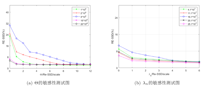
图2
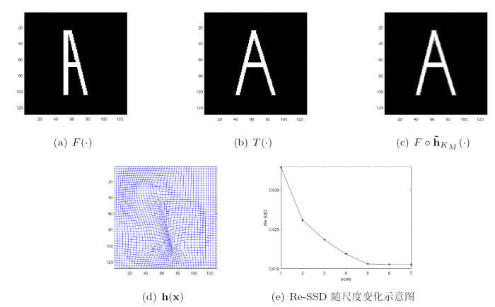
图3

图4
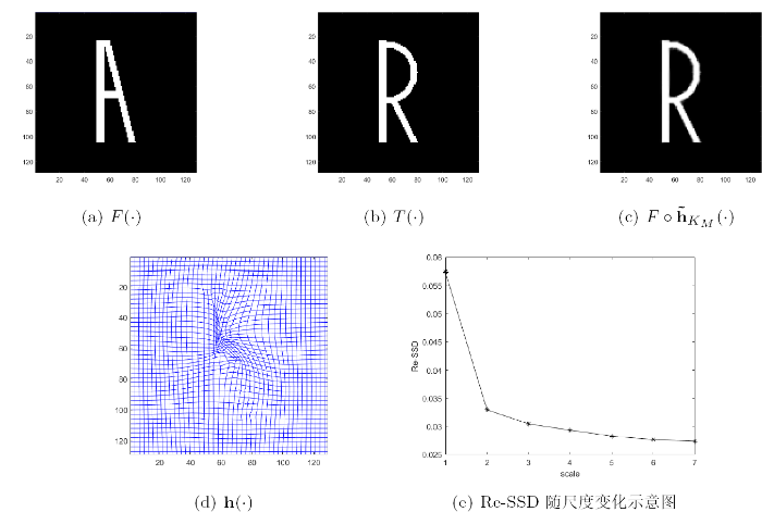
图5

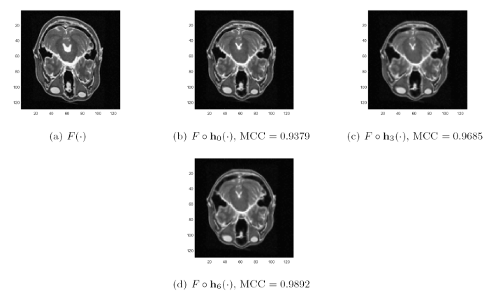
算法有效性检验 在进行多模态图像配准对比实验之前, 先用一组已知形变场的图像对来进行有效性测试. 如图6 所示,
图6
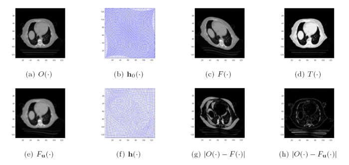
图7
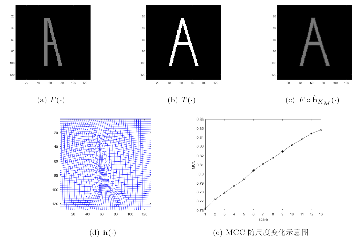
图8
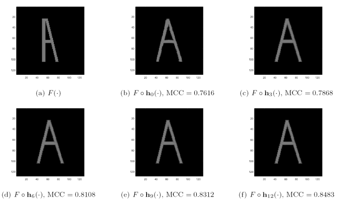
图9
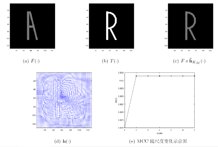
图10
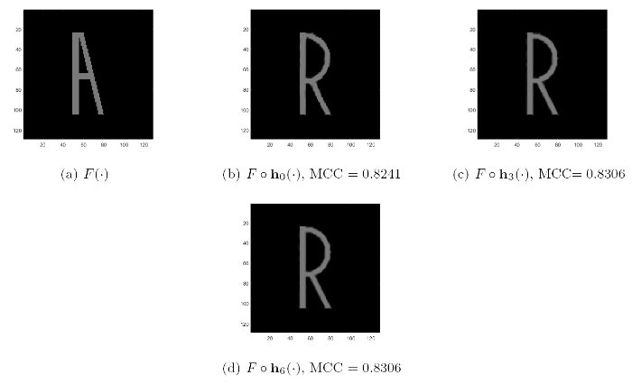
图11
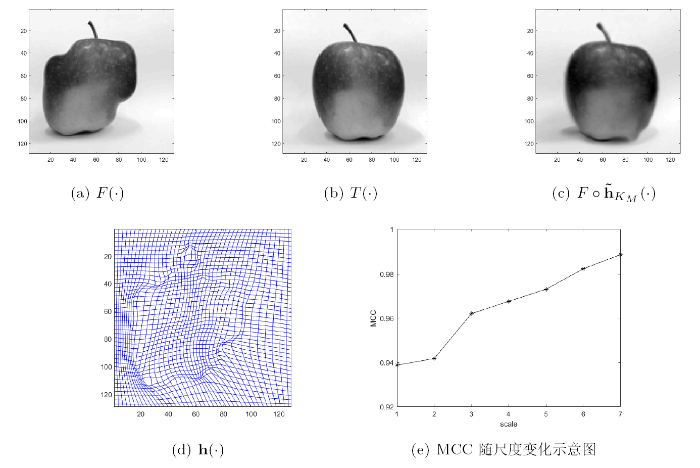
图12

图13
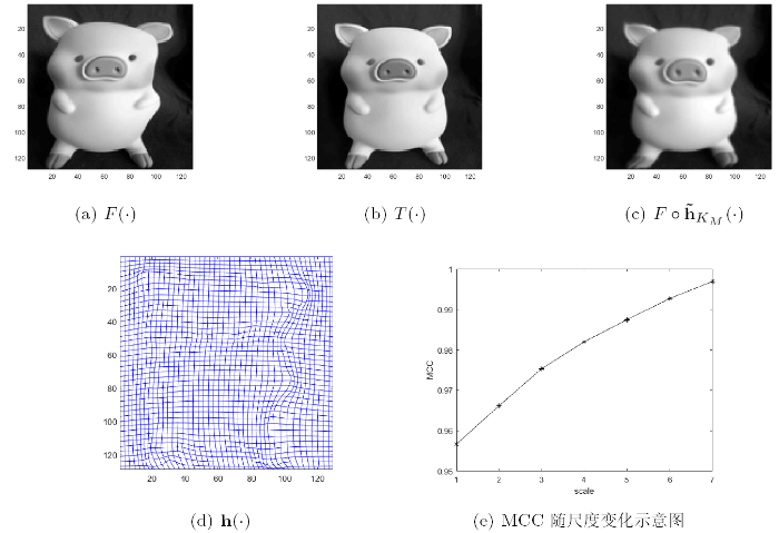
图14
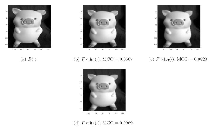
图15
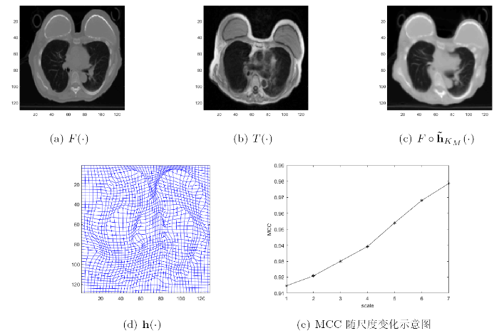
图16
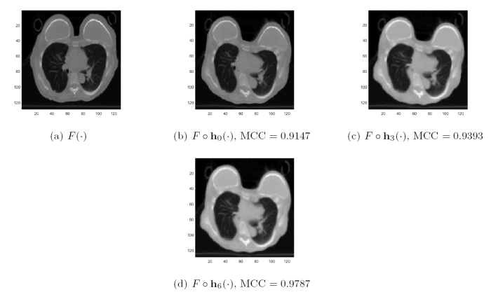
图17

图18
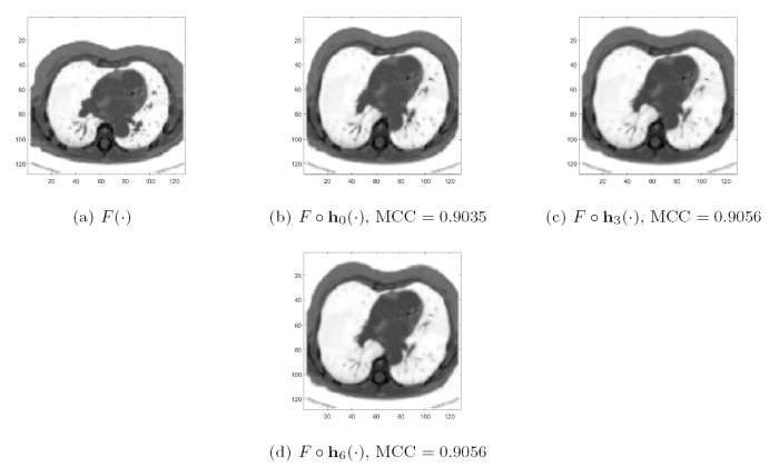
图19
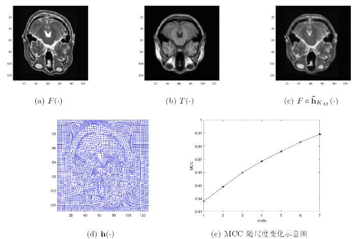
图20


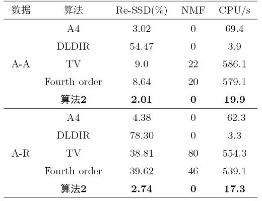
合成图像配准
自然图像配准
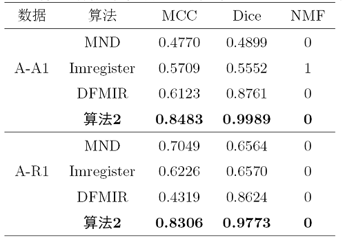
医学图像配准
从表4 三组医学图像的配准结果中可以看出, DFMIR 算法虽然配准结果较好, 但是有明显的网格重叠, 算法 2 有效地避免了网格重叠且配准效果较好, 说明了算法 2 在多模态医学图像配准中的有效性.
5 结论
本文在多模态图像配准中提出了一种基于瑞利度量的二维微分同胚多尺度算法, 有效地避免了网格重叠, 且实现了在没有先验正则项的情况下寻找二维微分多模态图像配准的最优解, 并通过具体的实验证明了算法在单模态和多模态图像配准中的有效性.
参考文献
Fast local trust region technique for diffusion tensor registration using exact reorientation and regularization
DOI:10.1109/TMI.2013.2274051
PMID:23880040
[本文引用: 1]

Diffusion tensor imaging is widely used in brain connectivity research. As more and more studies recruit large numbers of subjects, it is important to design registration methods which are not only theoretically rigorous, but also computationally efficient. However, the requirement of reorienting diffusion tensors complicates and considerably slows down registration procedures, due to the correlated impacts of registration forces at adjacent voxel locations. Based on the diffeomorphic Demons algorithm (Vercauteren, 2009), we propose a fast local trust region algorithm for handling inseparable registration forces for quadratic energy functions. The method guarantees that, at any time and at any voxel location, the velocity is always within its local trust region. This local regularization allows efficient calculation of the transformation update with numeric integration instead of completely solving a large linear system at every iteration. It is able to incorporate exact reorientation and regularization into the velocity optimization, and preserve the linear complexity of the diffeomorphic Demons algorithm. In an experiment with 84 diffusion tensor images involving both pair-wise and group-wise registrations, the proposed algorithm achieves better registration in comparison with other methods solving large linear systems (Yeo, 2009). At the same time, this algorithm reduces the computation time and memory demand tenfold.
Multimodality image registration by maximization of mutual information
DOI:10.1109/42.563664
PMID:9101328
[本文引用: 1]
A new approach to the problem of multimodality medical image registration is proposed, using a basic concept from information theory, mutual information (MI), or relative entropy, as a new matching criterion. The method presented in this paper applies MI to measure the statistical dependence or information redundancy between the image intensities of corresponding voxels in both images, which is assumed to be maximal if the images are geometrically aligned. Maximization of MI is a very general and powerful criterion, because no assumptions are made regarding the nature of this dependence and no limiting constraints are imposed on the image content of the modalities involved. The accuracy of the MI criterion is validated for rigid body registration of computed tomography (CT), magnetic resonance (MR), and photon emission tomography (PET) images by comparison with the stereotactic registration solution, while robustness is evaluated with respect to implementation issues, such as interpolation and optimization, and image content, including partial overlap and image degradation. Our results demonstrate that subvoxel accuracy with respect to the stereotactic reference solution can be achieved completely automatically and without any prior segmentation, feature extraction, or other preprocessing steps which makes this method very well suited for clinical applications.
Medical image registration using mutual information
DOI:10.1109/JPROC.2003.817864 URL [本文引用: 1]
Nonrigid coregistration of diffusion tensor images using a viscous fluid model and mutual information
In this paper, a nonrigid coregistration algorithm based on a viscous fluid model is proposed that has been optimized for diffusion tensor images (DTI), in which image correspondence is measured by the mutual information criterion. Several coregistration strategies are introduced and evaluated both on simulated data and on brain intersubject DTI data. Two tensor reorientation methods have been incorporated and quantitatively evaluated. Simulation as well as experimental results show that the proposed viscous fluid model can provide a high coregistration accuracy, although the tensor reorientation was observed to be highly sensitive to the local deformation field. Nevertheless, this coregistration method has demonstrated to significantly improve spatial alignment compared to affine image matching.
Multi-modal image registration by minimising Kullback-Leibler distance//International Conference on Medical Image Computing and Computer-Assisted Intervention
A new similarity measure for multi-modal image registration//IEEE International Conference on Image Processing
A novel high-order functional based image registration model with inequality constraint
DOI:10.1016/j.camwa.2016.10.018 URL [本文引用: 1]
A diffeomorphic image registration model with fractional-order regularization and Cauchy-Riemann constraint
DOI:10.1137/19M1260621 URL [本文引用: 3]
A fast multi grid algorithm for 2D diffeomorphic image registration model
A multiscale theory for image registration and nonlinear inverse problems
DOI:10.1016/j.aim.2019.02.014
[本文引用: 1]
In an influential paper, Tadmor et al. (2004) [42] introduced a hierarchical decomposition of an image as a sum of constituents of different scales. Here we construct analogous hierarchical expansions for diffeomorphisms, in the context of image registration, with the sum replaced by composition of maps. We treat this as a special case of a general framework for multiscale decompositions, applicable to a wide range of imaging and nonlinear inverse problems. As a paradigmatic example of the latter, we consider the Calderon inverse conductivity problem. We prove that we can simultaneously perform a numerical reconstruction and a multiscale decomposition of the unknown conductivity, driven by the inverse problem itself. We provide novel convergence proofs which work in the general abstract settings, yet are sharp enough to prove that the hierarchical decomposition of Tadmor, Nezzar and Vese converges for arbitrary functions in L-2, a problem left open in their paper. We also give counterexamples that show the optimality of our general results. (C) 2019 Published by Elsevier Inc.
Multi-scale approach for two-dimensional diffeomorphic image registration
DOI:10.1137/20M1383987 URL [本文引用: 4]
On measures of dependence
Diffeomorphic log demons image registration
Diffeomorphic demons: Efficient non-parametric image registration
DOI:10.1016/j.neuroimage.2008.10.040 URL [本文引用: 2]
A duality based algorithm for TV-
A combination of the total variation filter and a fourth-order filter for image registration
Multimodality non-rigid demon algorithm image registration
MRI modalitiy transformation in demon registration//IEEE International Symposium on Biomedical Imaging: From Nano to Macro
A coarse-to-fine deformable transformation framework for unsupervised multi-contrast MR image registration with dual consistency constraint
DOI:10.1109/TMI.2021.3059282
PMID:33577451
[本文引用: 1]
Multi-contrast magnetic resonance (MR) image registration is useful in the clinic to achieve fast and accurate imaging-based disease diagnosis and treatment planning. Nevertheless, the efficiency and performance of the existing registration algorithms can still be improved. In this paper, we propose a novel unsupervised learning-based framework to achieve accurate and efficient multi-contrast MR image registration. Specifically, an end-to-end coarse-to-fine network architecture consisting of affine and deformable transformations is designed to improve the robustness and achieve end-to-end registration. Furthermore, a dual consistency constraint and a new prior knowledge-based loss function are developed to enhance the registration performances. The proposed method has been evaluated on a clinical dataset containing 555 cases, and encouraging performances have been achieved. Compared to the commonly utilized registration methods, including VoxelMorph, SyN, and LT-Net, the proposed method achieves better registration performance with a Dice score of 0.8397± 0.0756 in identifying stroke lesions. With regards to the registration speed, our method is about 10 times faster than the most competitive method of SyN (Affine) when testing on a CPU. Moreover, we prove that our method can still perform well on more challenging tasks with lacking scanning information data, showing the high robustness for the clinical application.
