

1 引言
在许多物理问题, 以及天文学, 力学, 金融系统等领域, 我们经常遇到大量的非线性方程. 随着科学的不断发展, 对此类方程求出精确解问题受到人们的广泛关注. 目前已经有很多求精确解的方法[1-7], 其中Hirota双线性方法通常被认为是求解非线性方程组孤子解的一种简便而直接的方法. 近期, 马文秀教授提出了Hirota
2 z=x
方程(1.1)在维数约化
为便于求出方程(2.1)的双线性形式, 对方程(2.1)中的变量
其中
为了将上式转化成合适的
其中
根据贝尔多项式相关理论, (2.4)式可以写成如下
进一步, 在下面的变换下
可以得到方程(2.2)的双线性表示形式为
3 孤子解与呼吸波解
这一节, 先利用Hirota直接方法给出方程(1.1)的
其中
由文献[20]中所述, 对(3.2)和(3.3)式中取如下的参数约束, 可以获得方程(1.1)的
下面取定适当参数来刻画
则(3.2)式中
图 1
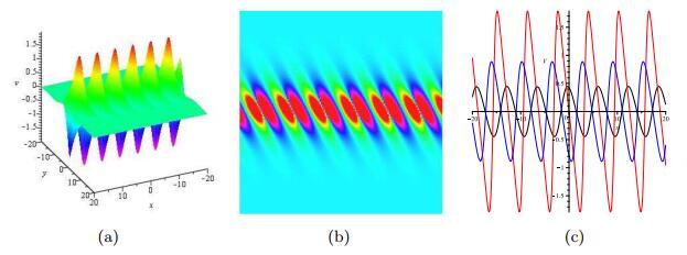
图 1
方程(1.1)的1-阶呼吸波解, 参数为(3.5)式. (a)
4 Lump波解
本节, 利用长波极限方法获得方程(1.1)的高阶lump波解. 对(3.2)式中的相位参数取
其中
且
值得注意的是为获得非奇异的lump波解, 参数
4.1 1-阶lump解
为获得
其中
在(4.5)式中对
则可以获得
其中
即
图 2
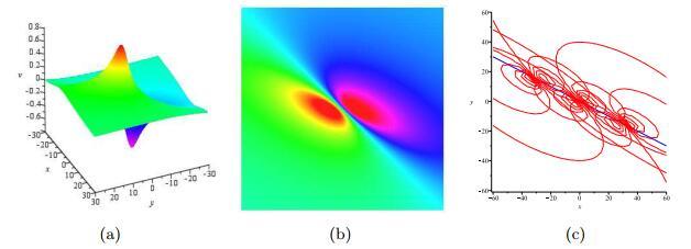
图 2
方程(1.1)的1-阶lump波解, 参数为
4.2 2-阶lump解
当
其中
取
从而有
其中
图 3
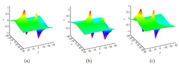
图 3
方程(1.1)的
5 半有理解
这一节, 对(3.2)式中的部分指数函数取长波极限从而获得方程(1.1)的半有理解. 即在(3.2)式中取
首先我们研究
其中
其中
图 4表示的是
图 4
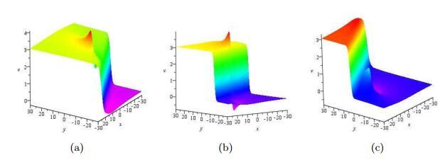
图 4
接下来我们研究2-阶lump解和单孤子解的混合解. 为此, 参数的选取为
其中
且
其中
图 5表示的是
图 5
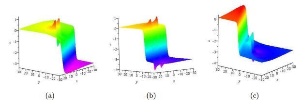
图 5
6 结论
该文研究了
参考文献
一类广义浅水波KdV方程的可积性研究
DOI:10.3969/j.issn.1003-3998.2019.03.005
The integrability of the KdV-shallow water wave equation
DOI:10.3969/j.issn.1003-3998.2019.03.005
Gaussian solitary wave solutions for nonlinear evolution equations with logarithmic nonlinearities
Generation of rogue waves in gyrotrons operating in the regime of developed turbulence
DOI:10.1103/PhysRevLett.119.034801
Rogue waves and their generating mechanisms in different physical contexts
DOI:10.1016/j.physrep.2013.03.001
Rogue waves of the nonlocal Davey-Stewartson I equation
DOI:10.1088/1361-6544/aac761 [本文引用: 1]
Soliton solutions to the B-type Kadomtsev-Petviashvili equation under general dispersion relations
DOI:10.1016/j.wavemoti.2021.102719 [本文引用: 1]
N-soliton solution of a combined pKP-BKP equation
DOI:10.1016/j.geomphys.2021.104191
N-soliton solutions and the Hirota conditionsin (1+1)-dimensions
N-soliton solutions and the Hirota conditions in (2+1)-dimensions
DOI:10.1007/s11082-020-02628-7
N-soliton solution and the Hirota condition of a (2+1)-dimensional combined equation
Lump solutions to the Kadomtsev-Petviashvili equation
DOI:10.1016/j.physleta.2015.06.061 [本文引用: 1]
Lump solutions to dimensionally reduced p-gKP and p-gBKP equations
Asymptotic behavior of a weakly dissipative modified two-component Dullin-Gottwald-Holm system
DOI:10.1016/j.aml.2018.03.019 [本文引用: 1]
Solitons and rational solutions of nonlinear evolution equations
Two-dimensional lumps in nonlinear dispersive systems
DOI:10.1063/1.524208 [本文引用: 1]
Lump solutions and interaction phenomenon for (2+1)-dimensional Sawada-Kotera equation
DOI:10.1088/0253-6102/67/5/473 [本文引用: 1]
Long-time asymptotic behavior for the Gerdjikov-Ivanov type of derivative nonlinear Schrodinger equation with time-periodic boundary condition
Rogue waves in the three-dimensional Kadomtsev-Petviashvili equation
DOI:10.1088/0256-307X/33/11/110201 [本文引用: 1]
Analysis on lump, lumpoff and rogue waves with predictability to the (2+1)-dimensional B-type Kadomtsev-Petviashvili equation
DOI:10.1016/j.physleta.2018.08.002
Dynamics of rogue waves on multi-soliton background in the Benjamin Ono equation
DOI:10.1007/s12043-016-1361-0 [本文引用: 1]
Doubly localized two-dimensional rogue waves in the Davey-Stewartson I equation
DOI:10.1007/s00332-021-09720-6 [本文引用: 1]
Completely resonant collision of lumps and line solitons in the Kadomtsev-Petviashvili I equation
Doubly localized rogue waves on a background of dark solitons for the Fokas system
DOI:10.1016/j.aml.2021.107435 [本文引用: 1]
Rational and semi-rational solutions of the nonlocal Davey-Stewartson equations
DOI:10.1111/sapm.12178 [本文引用: 1]
Resonant behavior of multiple wave solutions to a Hirota bilinear equation
DOI:10.1016/j.camwa.2016.06.008 [本文引用: 2]
Solitary waves, homoclinic breather waves and rogue waves of the (3+1)-dimensional Hirota bilinear equation
DOI:10.1016/j.camwa.2017.10.037 [本文引用: 2]
Study of lump dynamics based on a dimensionally reduced Hirota bilinear equation
DOI:10.1007/s11071-016-2755-8 [本文引用: 1]
Lump solution and integrability for the associated Hirota bilinear equation
DOI:10.1007/s11071-016-3216-0 [本文引用: 2]
