

1 引言
正交多项式是在19世纪末由Chebyshev对连分式的研究发展起来的. 随后有越来越多的数学家, Szegö, Bernstein, Akhiezer, Ismail等等, 对它进行研究. 正交多项式有很多有用的性质, 并且广泛应用于数学及数学物理中, 例如近似理论, 随机过程, 随机矩阵. 自20世纪60年代, Géza Freud开始研究正交于实数域
Freud[4]给出了关于权函数
它所对应的循环系数
朱孟坤等在文献[27]中构造了一类介于高斯权函数和四次Freud - 型权函数之间的权函数
设
根据正交条件, 可知
这里,
对正交于Freud - 型权函数(1.2)的多项式而言, 它们的三项循环递推关系式是
其中
且
另外,
将(1.4) 式带入(1.5) 式, 可以得到
关于十次Freud - 型权函数(1.2) 的矩定义为
这里
Hankel矩阵是随机矩阵中最基本的研究对象之一. 其行列式可以代表一个特定随机矩阵的配分函数, 或者可以代表一个随机变量与系综相关的母函数, 亦或者与最大特征值的分布有关. 在给定一个权函数的前提下, 最大或最小特征值的研究又可以提供有关Hankel矩阵非常有用的信息.
在本文第2、3节, 我们将分别给出权函数(1.2)所对应的循环系数
2 循环系数的行列式表达
定义两个新的Hankel行列式
和
它们和(1.8)式可以建立起这样的联系
与此同时, Freud -型权函数(1.2)作为定义在实数范围内恒正的对称函数, 所以
引理2.1 设
和
成立.
证 对于任一个非负整数
再结合
注2.1
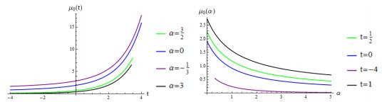
借助Mathematica软件, 我们可以用超几何函数
图 1
引理2.2 关于Freud - 型权函数(1.2)的Hankel行列式
证
对照(2.1) 和(2.2) 式, 即可得证(2.7)式.
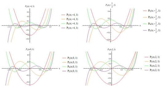
定理2.1 正交于Freud - 型权函数(1.2)的首一的正交多项式
这里
并且
证 根据(1.9)和(2.3)式, 有
用引理2.2, 代换上式的
另一方面, Vein和Dale[20]已经证明
那么
再结合引理2.2, 可得
至此, 得证(2.9)式. 同理可得(2.10)式.
图 2
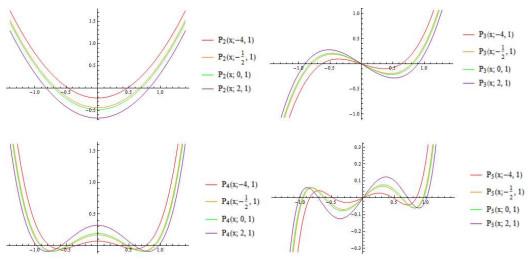
图 3
注2.2
3 循环系数满足的差分方程
定理3.1 对于(1.4) 式中的循环系数
证 为了方便起见, 记
这里
将(3.2) 和(3.3) 式带入到如下的积分计算中, 并结合(1.3) 式, 我们得到
另一方面
这里
注3.1 方程(3.1)是一个八阶差分方程, 属于离散的Painlevé I方程族, 可参考文献[22]. 类似地, 我们可称该方程为
4 循环系数的近似值
利用Freud[4]中的结论, 关于权函数
于是, 可以得到关于权函数(1.2)的循环系数
图 4
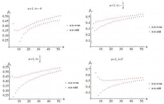
图 4
当
定理4.1 对于(1.4) 式中的循环系数
这里,
证 通过观察(3.1) 式,
这里通过(4.1)式, 可知
这就意味着,
和
进而
这里
定理4.1得证.
图 5

图 5
当
5 Hankel行列式满足的方程
定理5.1 关于Freud - 型权函数(1.2), 当
这里,
证 在(2.9) 和(2.10) 式的两边同时进行积分, 可得
和
联立(5.2) 和(5.3) 式, 并且在消去
其中
将(5.5) 和(5.6) 式代入(5.4) 式, 并且进行积分运算, 可得
6 Hankel矩阵的最小特征值
在这一节, 我们讨论由权函数
生成的Hankel矩阵的最小特征值在
接下来, 我们给出本文关于最小特征值的结论.
定理6.1 关于权函数(6.1), 它的最大Hankel矩阵所对应的最小特征值可以表示成
这里
于是
从而[24], 有
这个结果也对应了(4.1)式. 将(6.4) 式应用于(6.2)式, 有
这里
基于Chen和Lubinsky的理论[31], 同时利用
可以计算出最小特征值
定理6.1得证.
参考文献
On the coefficients in the recursion formulae of orthogonal polynomials
A proof of Freud's conjecture for exponential weights
DOI:10.1007/BF02075448 [本文引用: 1]
On Freud's equations for the exponential weights
DOI:10.1016/0021-9045(86)90088-2 [本文引用: 1]
A generalized Freud weight
DOI:10.1111/sapm.12105 [本文引用: 2]
Properties of generalized Freud polynomials
Semiclassical asymptotics of orthogonal polynomials: Riemann-Hilbert problem, and universality in the matrix model
Double scaling limit in the random matrix model: the Riemann-Hilbert approach
The relationship between semiclassical Laguerre polynomials and the fourth Painlevé equation
DOI:10.1007/s00365-013-9220-4 [本文引用: 1]
The largest eigenvalue distribution of the Laguerre unitary ensemble
DOI:10.1016/S0252-9602(17)30013-9 [本文引用: 1]
Global asymptotics of orthogonal polynomials associated with
DOI:10.1016/j.jat.2009.09.007 [本文引用: 1]
Estimates of the orthogonal polynomials with weight
DOI:10.1016/0021-9045(86)90074-2 [本文引用: 1]
Orthogonal polynomials and their derivatives I
DOI:10.1016/0021-9045(84)90023-6
Orthogonal polynomials with discontinuous weights
DOI:10.1088/0305-4470/38/12/L01 [本文引用: 1]
On semi-classical orthogonal polynomials associated with a Freud - type weight
DOI:10.1002/mma.6270 [本文引用: 1]
The discrete first, second and thirty-fourth Painlevé hierarchies
DOI:10.1088/0305-4470/32/4/009 [本文引用: 1]
Asymptotics of recurrence coefficients for orthonormal polynomials on the line-Magnus method revisited
Thermodynamic relations of the Hermitian matrix ensembles
DOI:10.1088/0305-4470/30/19/006 [本文引用: 2]
On the linear statistics of Hermitian random matrices
DOI:10.1088/0305-4470/31/4/005
Coulomb fluid, Painlevé transcendents and the information theory of MIMO systems
DOI:10.1109/TIT.2012.2195154 [本文引用: 1]
On properties of a deformed Freud weight
DOI:10.1142/S2010326319500047 [本文引用: 2]
Small eigenvalues of large Hankel matrices: The indeterminate case
DOI:10.7146/math.scand.a-14379 [本文引用: 1]
The smallest eigenvalue of Hankel matrices
Small eigenvalues of large Hankel matrices
DOI:10.1088/0305-4470/32/42/306
Smallest eigenvalues of Hankel matrices for exponential weights
DOI:10.1016/j.jmaa.2004.01.032 [本文引用: 4]
Computing the smallest eigenvalue of large ill-conditioned Hankel matrices
DOI:10.4208/cicp.260514.231214a
On some Hermitian forms associated with two given curves of the complex plane
DOI:10.1090/S0002-9947-1936-1501884-1
Small eigenvalues of large Hankel matrices
DOI:10.1090/S0002-9939-1966-0189237-7
The smallest eigenvalue of large Hankel matrices
The smallest eigenvalue of large Hankel matrices generated by a deformed Laguerre weight
DOI:10.1002/mma.5583
Smallest eigenvalue of large Hankel matrices at critical point: Comparing conjecture with parallelised computation
The smallest eigenvalue of large Hankel matrices generated by a singularly perturbed Laguerre weight
DOI:10.1063/1.5140079 [本文引用: 1]
