

1 引言
最近, Sultana和Schlickeiser[15]考虑了三元ADRQP, 其包含未简并的冷移动重离子流(电荷
在本文中, 我们考虑无量纲的重离子声波, 其中惯性(恢复力)由重离子的质量密度(电子和轻离子的简并压力)提供, 满足下述方程
其中, 数密度
其中
为了研究方程(1.4)的行波解, 我们令
其中
在小幅波近似的假设下(即
对应Sagdeev势
其中,
本文的结构如下:在第2节中, 讨论了系统(1.7)的相图分岔与马赫数
2 相图的分岔
现在, 我们考虑系统(1.7)的相图可能的分岔. 为了研究系统(1.7) 的平衡点
由文献[20-22], 我们令
图 1
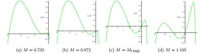
图 2
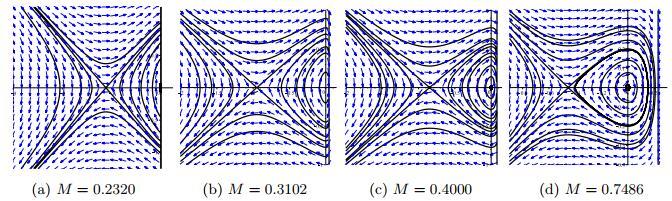
图 3
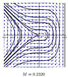
图 4
3 行波解的动力学行为
其中,
4 当原点为中心时精确行波解的参数表示
本节, 我们考虑参数
(1) 考虑马赫数
(i) 当
图 5
(ii) 当
(iii) 当
其中,
(2) 下面, 我们考虑马赫数
图 6
其中,
(ii) 对应水平曲线
其中,
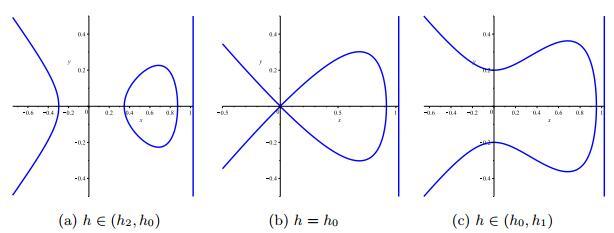
(3) 设马赫数
(i) (1.8) 的水平曲线定义为
左边的周期轨道族是包围平衡点
图 7
其中,
对应于过
(ii) 当
(4) 考虑马赫数
(i) 当
(ii) 当
其中,
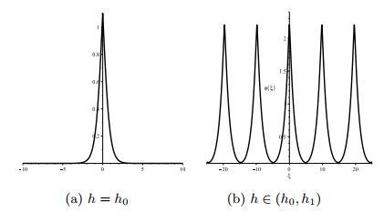
5 原点为尖点时精确行波解的参数表示
首先, 从图 3中, 我们注意到平衡点
6 原点为鞍点时精确行波解的参数表示
在本节中, 我们使用奇异行波系统理论来分析系统(1.7)的解函数
(1) 基于能量水平
(i) 考虑图 8(a). 在这种情况下, 当
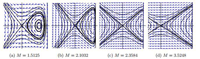
图 8
与过
其中,
(ii) 从图 8(b)可见, 由
其中,
此外, 在平衡点
其中,
(iii) 考虑图 8(c). 在这种情况下, 对于
其中,
(2) 在此情形下,
在本节中, 完全位于奇异直线
(i) 对于由
图 9
其中,
(ii) 对应于由
7 结论
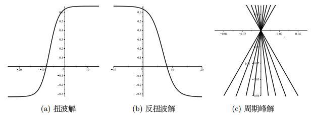
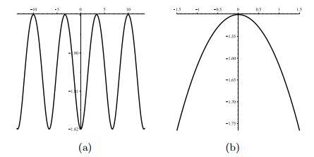
通过使用动力系统方法, 我们获得了十四个精确的显式行波解, 它们由双曲函数和雅可比椭圆函数表示. 其中, (4.6) 和(6.1) 式是周期波解, (4.8) 式是孤立波解, (4.1), (4.2), (4.3), (4.7), (6.2) 和(6.6) 式是紧性波解, (4.5) 式是周期峰波解, (4.4), (6.4)和(6.5) 式是扭波和反扭波解, (6.7)式是伪峰波解. 在每种情况下, 我们都使用Maple软件获得了一些解的波动曲线. 据此, 我们得出方程(1.1) 有周期解、周期的峰解、光滑的孤波解、伪峰解和紧性波解.
参考文献
Nonlinear collective effects in photon-photon and photon-plasma interactions
DOI:10.1103/RevModPhys.78.591 [本文引用: 1]
Extreme states of matter on Earth and in space
DOI:10.3367/UFNe.0179.200906h.0653
Dynamical instability of gaseous masses approaching the Schwarzschild limit in general relativity
Black holes, naked singularities and cosmic censorship
Dense Plasmas in astrophysics: from gaint planets to neuron stars
DOI:10.1088/0305-4470/39/17/S16 [本文引用: 2]
Electrostatic solitary waves in a quantum plasma with relativistically degenerate electrons
Solitary waves and double layers in an ultra-relativistic degenerate dusty electron-positron-ion plasma
Nonlinear ion acoustic excitations in relativistic degenerate, astrophysical electron-positron-ion plasmas
DOI:10.1017/S0022377813000524 [本文引用: 1]
Electrostatic solitary waves in relativistic degenerate electron-positron-ion plasma
DOI:10.1109/TPS.2015.2404298 [本文引用: 1]
Ion acoustic solitary waves in degenerate electron-ion plasmas
DOI:10.1109/TPS.2016.2539258 [本文引用: 1]
Ion acoustic shock waves in a degenerate relativistic plasma with nuclei of heavy elements
DOI:10.1140/epjp/i2017-11367-2 [本文引用: 1]
Ultra-low frequency shock dynamics in degenerate relativistic plasmas
Heavy nucleus-acoustic spherical solitons in self-gravitating super-dense plasmas
DOI:10.1063/1.4981262 [本文引用: 1]
Fully nonlinear heavy ion-acoustic solitary waves in astrophysical degenerate relativistic quantum plasmas
DOI:10.1007/s10509-018-3317-y [本文引用: 5]
Cooperative phenomena and shock waves in collisionless plasmas
One-soliton shaping and inelastic collision between double solitons in the fifth-order variable-coefficient Sawada-Kotera equation
DOI:10.1007/s11071-019-04866-1 [本文引用: 1]
Bifurcations and dynamical analysis of Coriolis-stabilized spherical lagging pendula
DOI:10.1007/s11071-019-04830-z
On a class of singular nonlinear traveling wave equations
DOI:10.1142/S0218127407019858 [本文引用: 2]
Travelling wave solutions and soliton solutions for the nonlinear transmission line using the generalized Riccati equation mapping method
Dynamics analysis and Hamilton energy control of a generalized Lorenz system with hidden attractor
DOI:10.1007/s11071-018-4539-9 [本文引用: 1]
Understanding peakons, periodic peakons and compactons via a shallow water wave equation
DOI:10.1142/S0218127416502072 [本文引用: 1]
Dynamical behavior and exact solution in invariant manifold for a septic derivative nonlinear Schrödinger equation
DOI:10.1007/s11071-017-3468-3 [本文引用: 1]
