

1 引言
通常在传染病模型中考虑潜伏期时,引入变量感染持续时间
其中
考虑到模型的现实意义,假设
这里
其中
根据上述的分析,本文提出一类具有接种和非线性感染率的时滞传染病模型
这里
考虑模型的现实意义,模型(1.7)的初值条件如下
其中
本文的其余部分安排如下.在第二节中,得到模型的基本再生数,并研究了地方病平衡点的存在性和系统解的非负性以及有界性.第三节利用特征方程研究了两个平衡点的局部稳定性.在第四节中,我们讨论了系统(1.7)的一致持续性.在第五节中,通过构建合适的Lyapunov泛函和应用Lyapunov-LaSalle不变性原理,我们分别获得了无病平衡点和地方病平衡点的全局渐近稳定性.最后,我们给出了一些数值拟合对理论结果进行了检验.
2 预备知识
易知模型(1.7)总存在一个无病平衡点
定理2.1 如果
证 由模型(1.7)的第一个和第二个方程知,可将
将(2.2)和(2.3)式代入模型(1.7)的第三个方程,得
这里
当
当
和
易知
定理2.2 模型(1.7)在初始条件(1.8)下的解是非负和有界的.
证 首先,我们证明
根据比较原理有
对
和
对
再次利用比较原理
接下来证明
易知
与假设矛盾.因此
3 平衡点的局部稳定性
为了研究模型(1.7)的局部稳定性,首先对模型(1.7)在平衡点
定理3.1 如果
证 特征方程(3.1)在
方程(3.2)有三个根
假设
分离上面方程右端的实部和虚部,然后平方相加得
显然当
当
定理3.2 如果
证 在
利用(2.2)和(2.3)式得
注意
利用(3.7)式, (3.8)式和
不妨假设
则有
这和等式(3.5)矛盾,意味着特征方程(3.5)的根不可能有非负实部,于是
4 系统(1.7)的一致持续性
定义4.1[17] 系统(1.7)是一致持续的是指:如果正存在
定理4.1 如果
证 根据定理2.2易知
和
当
对于任意
于是存在一个足够大的常数
同理可得
存在一个足够大的常数
令
和
我们断言
于是
类似地,当
当
由(4.2)式得
令
我们断言
和假设矛盾.因此,对所有的
这意味着当
和(4.9)式矛盾.因此,对所有
对于足够大的
如果
则当
如果
有
这和以上假设矛盾,意味着对所有的
5 平衡点的全局稳定性
定理5.1 如果
证 定义如下的Lyapunov泛函
这里
易得
利用等式
易知当
定理5.2 如果
证 定义如下的Lyapunov泛函
这里
易得
利用等式
和
有
显然,
6 数值模拟
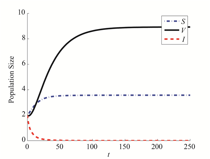
对于系统(1.7),我们选取参数值:
图 1
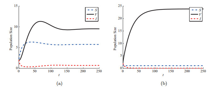
其次,选择
图 2
参考文献
Qualitative analysis and optimal control of an epidemic model with vaccination and treatment
DOI:10.1016/j.matcom.2013.11.005 [本文引用: 1]
On the definition and the computation of the basic reproduction ratio R_0 in models for infectious diseases in heterogeneous populations
A qualitative study of a vaccination model with nonlinear incidence
DOI:10.1016/S0096-3003(02)00372-7 [本文引用: 1]
Global stability analysis of an SVEIR epidemic model with general incidence rate
Global stability for delay SIR and SEIR epidemic models with nonlinear incidence rate
Global properties for virus dynamics model with Beddington-DeAngelis functional response
Persistence in infinite-dimensional systems
Global stability of a multi-group SVIR epidemic model
DOI:10.1016/j.nonrwa.2012.09.004 [本文引用: 1]
Global dynamics of delay epidemic models with nonlinear incidence rate and relapse
DOI:10.1016/j.nonrwa.2010.06.001 [本文引用: 1]
Dynamical behavior of epidemiological models with nonlinear incidence rates
DOI:10.1007/BF00277162 [本文引用: 1]
SVIR epidemic models with vaccination strategies
Seir epidemiological model with varying infectivity and infinite delay
The stability analysis of an SVEIR model with continuous age-structure in the exposed and infectious classes
DOI:10.1080/17513758.2015.1006696
Sveir epidemiological model with varying infectivity and distributed delays
Analysis of an SVEIR model with age-dependence vaccination, latency and relapse
DOI:10.22436/jnsa.010.07.31 [本文引用: 1]
Global dynamics for an age-structured epidemic model with media impact and incomplete vaccination
DOI:10.1016/j.nonrwa.2016.04.009 [本文引用: 1]
A possible association of Y chromosome heterochromatin with stature
DOI:10.1007/BF00294920 [本文引用: 1]
Global behavior and permanence of SIRS epidemic model with time delay
DOI:10.1016/j.nonrwa.2007.03.010 [本文引用: 1]
