


引言
并行磁共振成像(Parallel Magnetic Resonance Imaging,PMRI)[4⇓-6]技术采用多个接收线圈同时采集数据,可以有效减少成像时间.当加速因子R=1时,PMRI是对k空间数据进行全采样;而R>1时,则是对k空间数据进行欠采样.这虽然减少了采样时间,但是会得到混叠伪影的磁共振图像.图像重建可以有效抑制混叠伪影.典型的并行磁共振重建算法有GRAPPA(Generalized Auto-calibrating Partially Parallel Acquisitions)[7]、SENSE(Sensitivity Encoding)[8]、SPIRiT(Iterative Self-consistent Parallel Imaging Reconstruction)[9]等,但是当加速因子较大时,利用这些算法重建的图像质量会显著下降.
由于采集的是k空间的复数数据,因此经过傅里叶重建之后的磁共振图像也是复数图像.利用实数卷积神经网络进行磁共振图像重建可能会丢失相位信息,而由相位信息可以获知血流速度、血流流量、定量磁化图等,因此利用复数卷积神经网络进行快速MRI研究具有重要意义.基于复数模块的复数卷积神经网络研究开始于2017年,鉴于复数有更加丰富的表征能力,Trabelsi等[19]设计了基于复数网络的模块.2018年,Dedmari等[20]将复数相关模块应用于多线圈磁共振图像的重建中,提出了复数密集全卷积神经网络CDFNet,并且证明它在恢复图像精细结构和高频纹理方面有很大优势.2020年,Liang等[21]提出了一种基于拉普拉斯金字塔的复数神经网络框架CLP-Net用于单线圈快速MRI研究,该框架包含一个具有复数卷积和数据一致性层的级联多尺度网络结构,实验结果表明,该方法在定性和定量指标上都取得了很好的重建效果.基于复数卷积神经网络的快速多通道MRI方法目前属于起步阶段,2020年,Wang等[22]提出了深度残差复数卷积神经网络DeepcomplexMRI用于加速PMRI,并加入了k空间数据一致性操作,该网络使用大量现有的全采样多通道数据作为目标数据,结合相应的欠采样数据进行训练,实验结果表明,在相同的加速因子下,该方法可以产生更少的噪声和伪影.
PCU-Net(Parallel Complex U-Net)算法利用复数模块将单通道实数U型卷积神经网络拓展到多通道复数U型卷积神经网络[23],进行多通道欠采样数据的磁共振图像重建,在加速因子比较大时,PCU-Net也能对欠采样图像进行高质量重建.为了简化PCU-Net的网络结构、减少网络参数总量以加快网络训练速度,本文提出了基于PCAU-Net(Parallel Complex Asymmetric U-Net)的快速多通道MRI方法.通过对PCU-Net的网络结构进行简化,设计了一种结构不对称的复数U型网络结构,通过在解码部分减小网络规模以降低模型的复杂度;然后在跳跃连接前加入了1×1复数卷积以实现跨通道信息交互;在输入输出之间加入了残差连接为误差的反向传播提供捷径.实验结果表明,在规则和随机两种采样模式下,在使用不同加速因子进行采样时,相比PCU-Net的网络,PCAU-Net的网络参数减少了915 kB;训练时间缩短了约11.1%;相比经典的并行磁共振图像重建算法GRAPPA和SPIRiT,PCAU-Net重建质量显著升高.
1 PCAU-Net网络架构
1.1 PCAU-Net的网络模型
图1
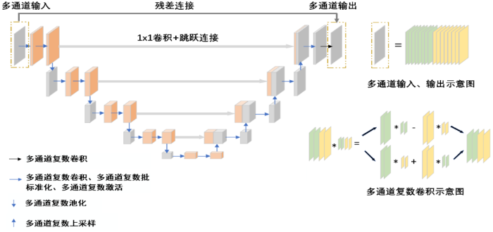
PCAU-Net网络包括4个下采样层和4个上采样层,其中下采样层包括多通道复数卷积、多通道复数批标准化、多通道复数激活和多通道复数池化;上采样层包括多通道复数卷积、多通道复数批标准化、多通道复数激活和多通道复数上采样.在每一个上采样层中,上采样输出和对应的下采样层输出进行通道维度上的拼接,在拼接前下采样层输出经过了一次1×1卷积,利用1×1卷积可以进行降维或者升维,在这里1×1卷积的主要作用是对各通道像素之间进行线性组合,实现跨通道信息交互[25,26].此外,PCAU-Net网络在输入和输出之间进行了残差连接,残差连接可以避免网络过深时性能的退化问题,同时也为误差的反向传播提供了捷径[27].
1.2 PCAU-Net的网络模块
1.2.1 多通道复数卷积
多通道复数卷积是将输入特征的实数部分和虚数部分分别进行卷积,如(1)式所示:
其中,*表示卷积;m、n分别表示通道数和层数;
其中,
1.2.2 多通道复数批标准化
批标准化是通过改变数据的均值和方差,增强模型的非线性表达能力,可以加快网络训练,防止过拟合.然而,常规的批标准化操作仅适用于实数数据,对于复数数据而言,可使用复数批标准化操作[19],将复数数据经过处理后成为标准正态复数分布,使得沿实部和虚部有相等的方差,从而确保它们之间的协同关系.多通道复数批标准化是在每个通道分别进行复数批标准化操作.
1.2.3 多通道复数激活函数
激活函数通过引入非线性因素,有效提升了模型的表达能力.本文选取modReLU作为复数激活函数.modReLU激活函数在原点创建半径为
其中,
1.2.4 多通道复数池化和复数上采样
多通道复数池化是对每个通道采用复数幅值最大值池化,将窗口内幅值最大的复数作为复数池化的结果.上采样的作用是放大图像,选取双线性插值算法作为复数上采样方法.多通道复数上采样是对每个通道采用双线性插值算法.
2 基于PCAU-Net的快速多通道磁共振图像重建
2.1 数据采集和预处理
实验数据下载地址为
原始的全采样k空间数据为
欠采样k空间数据由
其中, 表示对应像素点相乘,
将对应的多通道全采样和欠采样图像在每个通道分别进行复数数据归一化操作,即在保留每个通道复数数据原始相位的情况下对幅值进行归一化,然后将每个通道归一化后的幅值和保留的相位重新组合成多通道复数数据,具体计算如(9)式和(10)式所示.
其中,
2.2 网络的训练和参数设置
网络输入层起始卷积核个数为32,经过两次相同的卷积;4个下采样层卷积核个数分别为64、128、256、256,每层经过两次相同的卷积;4个上采样层卷积核个数分别为128、64、32、32,每层只经过一次卷积;输出层是8个1×1的卷积核,步长为1,填充(padding)为0;在多通道复数池化中,设置池化窗口大小为(2,2)、步长为2,获得原来数据尺寸一半的数据;在多通道复数上采样中,使用双线性插值作为上采样算法,比例因子为2,获得原来数据尺寸两倍的数据.
将训练集数据输入到PCAU-Net网络中,计算训练集全采样图像与网络输出值的损失值,损失函数采用多通道复数均方误差函数,在训练过程中使用验证集验证误差.多通道复数均方误差函数是在计算多通道复数数据误差时,对多通道数据的实部与虚部分别计算均方误差后再加权平均,得到最终的损失值loss,计算公式如(11)式所示:
其中
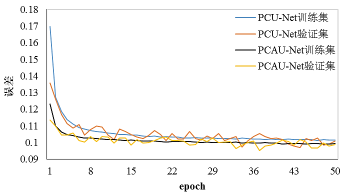
利用误差的反向传播机制和Adam优化器进行循环迭代优化,更新神经网络的参数θ.batch-size设置为2,Adam优化器参数配置(β1=0.9,β2=0.99),初始学习率设为0.005,以后每个epoch的学习率的指数衰减率为0.99.本文设置epoch为50,在加速因子R(N=5, C=32)=3.3的情况下,PCU-Net和PCAU-Net的训练集和验证集上的误差曲线如图2所示.从图中训练集误差曲线可以看出,训练到第50个epoch时,两个神经网络模型已经收敛,验证集误差曲线在各自神经网络的训练集误差曲线上下波动,网络收敛情况正常,根据验证集误差曲线的最小值选取最优网络参数.
图2
2.3 数据一致性保障和图像的重建
把测试集中的多通道欠采样图像
对网络的预测图像在k空间进行数据一致性操作可以提高重建图像的质量,首先对每个通道的预测图像进行离散傅里叶变换(Discrete Fourier Transform,DFT)得到k空间数据
再用实际采集的k空间数据替换
2.4 量化指标
通过总相对误差(Total Relative Error,TRE)、结构相似性(Structural Similarity,SSIM)[28]、峰值信噪比(Peak Signal to Noise Ratio,PSNR)三个计算指标对重建图像进行定量分析,重建图像的TRE越小、SSIM和PSNR越大,说明重建图像质量越好.其中,TRE的计算公式如(15)式所示:
其中,
3 结果与讨论
3.1 上采样方法的对比
表1 基于规则采样,R (N = 5, C = 32) = 3.3时,分别使用双线性插值和反卷积进行上采样的PCAU-Net的量化指标
Table 1
| 量化指标 | 双线性插值 | 反卷积 |
|---|---|---|
| TRE | 8.98×10⁻⁴ | 9.02×10⁻⁴ |
| SSIM | 0.9787 | 0.9795 |
| PSNR | 32.1041 | 32.2539 |
| 参数量/kB | 25359 | 36249 |
sampling with R (N = 5, C = 32) = 3.3
3.2 基于规则采样的不同网络架构的对比
3.2.1 不同算法单通道重建图像的对比
图3为在加速因子R (N = 5, C = 32) = 3.3时,100张8通道测试数据中的一张复数膝盖数据中的其中一个通道(第5个通道,共有8个通道)的重建幅值图和相位图,以及各自的局部放大图和局部误差放大图,其中误差是指重建图像与参考图之间的误差.从幅值放大图箭头所示处可见,GRAPPA重建幅值图中有明显的伪影,而PCU-Net和PCAU-Net伪影较少;从误差放大图来看,GRAPPA的误差最大,PCAU-Net的幅值误差较小.从相位放大图箭头所示处可见,GRAPPA相位放大图中有较多的伪影,而PCU-Net和PCAU-Net伪影较少;从相位误差放大图中可以看出GRAPPA的相位误差最大,PCU-Net和PCAU-Net的相位误差接近.在图3的第5通道数据重建图中,GRAPPA的PSNR、SSIM和TRE值分别为20.929 6、0.824 9和2.70×10⁻³,PCU-Net重建图像的PSNR、SSIM和TRE值分别为30.735 8、0.984 7和9.64×10⁻⁴,PCAU-Net重建图的PSNR、SSIM和TRE值分别为31.735 8、0.991 9和8.35×10⁻⁴.从量化指标来看,PCAU-Net重建图的质量比GRAPPA和PCU-Net更高.
图3
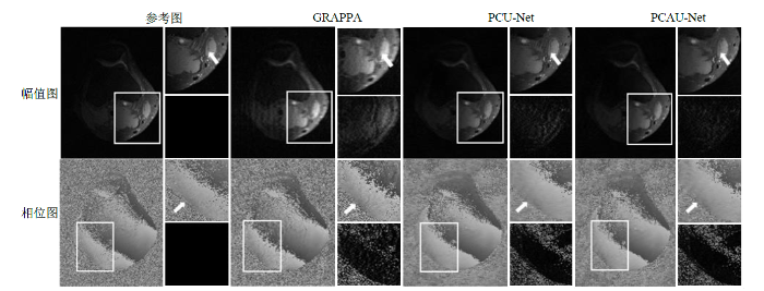
图3
基于规则采样,R (N = 5, C = 32) = 3.3时,第5个通道的幅值和相位的重建图(每幅图左侧)、局部放大图(每幅图右上)、局部误差放大图(每幅图右下)
Fig. 3
Reconstructed amplitude and phase maps (left in each figure), and their local enlarged maps (upper right in each figure) and local error enlarged maps (lower right in each figure) of the fifth channel based on regular sampling with R (N = 5, C = 32) = 3.3
3.2.2 不同算法多通道数据重建图像的对比
加速因子R (N = 5, C = 32) = 3.3时,在100张8通道测试数据中取出一张复数膝盖数据经过GCC合成后,GRAPPA、PCU-Net和PCAU-Net的最终幅值和相位重建图像,以及各自的放大图和误差放大图如图4所示,可以看出经多通道数据重建后的图像质量显著提升,图像中没有线圈位置摆放所造成的单个通道的明暗差异.从图4箭头所示处可见,GRAPPA幅值放大图中有明显的伪影,而PCU-Net和PCAU-Net可显著地抑制伪影;从幅值误差放大图也可以看出GRAPPA的幅值误差最大,PCAU-Net的幅值误差最小.从相位图箭头所示处可见,GRAPPA相位放大图中有明显伪影,而PCU-Net和PCAU-Net显著抑制了伪影;从相位误差放大图中可以看出GRAPPA的相位误差最大,PCU-Net和PCAU-Net的相位误差接近,均小于GRAPPA.图4多通道数据重建图中,GRAPPA重建图的PSNR、SSIM和TRE值分别为26.372 8、0.911 2和1.80×10⁻³,PCU-Net重建图的PSNR、SSIM和TRE值分别为30.660 8、0.959 8和9.64×10⁻⁴,PCAU-Net重建图的PSNR、SSIM和TRE值分别为31.913 3、0.972 7和8.35×10⁻⁴.可以看出,GRAPPA重建图的客观量化指标比较差,且与PCU-Net和PCAU-Net重建图有较大差距,而PCAU-Net重建图的客观量化指标在三者中最优.
图4

图4
基于规则采样,R (N = 5, C = 32) = 3.3时,多通道的幅值和相位的重建图(每幅图左侧)、局部放大图(每幅图右上)、局部误差放大图(每幅图右下)
Fig. 4
Reconstructed amplitude and phase maps (left in each figure), and their local enlarged maps (upper right in each figure) and local error enlarged maps (lower right in each figure) of the multi-channels based on regular sampling with R (N = 5, C = 32) = 3.3
3.2.3 不同网络架构客观量化指标的对比
基于规则采样,在不同加速因子下,不同算法重建的100张测试图像各定量指标的平均值如表2所示.当R (N=3, C=32) = 2.5时,GRAPPA和PCU-Net、PCAU-Net的SSIM、PSNR值的差距较小.但是当R (N=12, C=32) = 5.0时,PCU-Net和PCAU-Net的SSIM值都仍然保持在0.942以上,而GRAPPA则只有0.812 5;PCU-Net和PCAU-Net的PSNR值都仍然保持在28.7以上,而GRAPPA则只有22.555 9.由此可见,GRAPPA这种经典的PMRI算法只有在加速因子较小时才能获得较好的重建效果,当加速因子较大时,其重建质量显著下降;而PCAU-Net网络和PCU-Net网络无论在低加速因子还是在高加速因子情况下,重建图像质量都要优于GRAPPA.虽然在加速因子R (N=9, C=32)=4.6时,PCU-Net重建图像的SSIM略高于PCAU-Net,在加速因子R (N=12, C=32)=5.0时,PCU-Net重建图像的PSNR略高于PCAU-Net,但是在其余几种加速因子下,PCAU-Net重建图像的PSNR、SSIM均更高,并且TRE更低,这说明PCAU-Net相比于PCU-Net,虽然在解码部分进行了网络简化,但是这种简化并不会带来网络性能的大幅度退化,并且由于残差连接的引入和对跳跃连接的优化,使得简化后的PCAU-Net网络能够重建出质量更高的图像.
表2 基于规则采样,在不同加速因子下,不同算法重建图像的定量指标的平均值
Table 2
| 量化指标 | GRAPPA | PCU-Net | PCAU-Net | ||||
|---|---|---|---|---|---|---|---|
| TRE | R (N=3, C=32)=2.5 | 1.10×10⁻³ | 8.08×10⁻⁴ | 7.64×10⁻⁴ | |||
| R (N=5, C=32)=3.3 | 1.80×10⁻³ | 9.44×10⁻⁴ | 8.98×10⁻⁴ | ||||
| R (N=7, C=32)=4.0 | 2.40×10⁻³ | 9.73×10⁻⁴ | 9.33×10⁻⁴ | ||||
| R (N=9, C=32)=4.6 | 2.60×10⁻³ | 1.70×10⁻³ | 1.40×10⁻³ | ||||
| R (N=12, C=32)=5.0 | 2.90×10⁻³ | 1.70×10⁻³ | 1.70×10⁻³ | ||||
| SSIM | R (N=3, C=32)=2.5 | 0.9645 | 0.9758 | 0.9787 | |||
| R (N=5, C=32)=3.3 | 0.9123 | 0.9673 | 0.9701 | ||||
| R (N=7, C=32)=4.0 | 0.8634 | 0.9669 | 0.9688 | ||||
| R (N=9, C=32)=4.6 | 0.8337 | 0.9627 | 0.9543 | ||||
| R (N=12, C=32)=5.0 | 0.8125 | 0.9422 | 0.9424 | ||||
| PSNR | R (N=3, C=32)=2.5 | 30.4921 | 33.0363 | 33.5118 | |||
| R (N=5, C=32)=3.3 | 26.0461 | 31.6888 | 32.1041 | ||||
| R (N=7, C=32)=4.0 | 23.6166 | 31.4050 | 31.7779 | ||||
| R (N=9, C=32)=4.6 | 22.9207 | 29.5721 | 30.7301 | ||||
| R (N=12, C=32)=5.0 | 22.5559 | 28.7280 | 28.7139 | ||||
注:黑体表示最优指标数据.
3.2.4 不同算法的统计优势对比
当加速因子R (N=5, C=32) = 3.3时,GRAPPA的TRE最大,SSIM和PSNR最小,重建效果最差;PCAU-Net和PCU-Net的重建效果显著优于GRAPPA,而且PCAU-Net和PCU-Net的重建效果虽然接近,但是PCAU-Net在各指标上还是略优于PCU-Net(图5).
图5
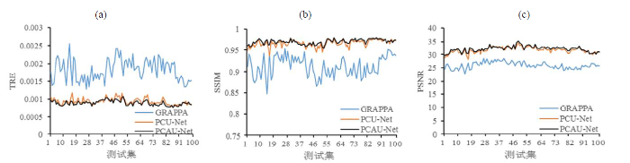
图5
基于规则采样,加速因子R (N=5, C=32) = 3.3时,GRAPPA、PCU-Net和PCAU-Net重建的测试集图像的量化指标图示.(a) TRE;(b) SSIM;(c) PSNR
Fig. 5
Quantitative values of testing images with GRAPPA, PCU-Net and PCAU-Net reconstructions based on regular sampling with R (N=5, C=32) = 3.3. (a) TRE; (b) SSIM; (c) PSNR
为了更清楚地比较PCAU-Net相对于PCU-Net的优势,本文对PCAU-Net重建图像量化指标优于PCU-Net重建图像的数量占所有测试集图像(100张)的比例进行了统计.如表3所示,基于规则采样,在加速因子R (N=3, C=32) = 2.5、R (N=5, C=32) = 3.3、R (N=7, C=32) = 4.0时,PCAU-Net重建图像的质量量化指标优势远大于PCU-Net,而在R (N=9, C=32) = 4.6时,PCAU-Net的SSIM指标优势略低于PCU-Net,在 R (N=12, C=32) = 5.0时,两者的指标优势差别不显著.
表3 基于规则采样,不同加速因子下,PCAU-Net重建图像相对于PCU-Net重建图像量化指标优势的统计
Table 3
| 量化指标 | R (N=3, C=32) = 2.5 | R (N=5, C=32) = 3.3 | R (N=7, C=32) = 4.0 | R (N=9, C=32) = 4.6 | R (N=12, C=32) = 5.0 |
|---|---|---|---|---|---|
| TRE | 91% | 86% | 86% | 79% | 48% |
| SSIM | 88% | 84% | 75% | 44% | 53% |
| PSNR | 91% | 86% | 86% | 61% | 52% |
表中数据为PCAU-Net重建图像量化指标优于PCU-Net重建图像的数量占所有测试集图像(100张)的比例.
images based on regular sampling with different acceleration factors
3.3 基于随机采样的不同网络架构的对比
3.3.1 不同算法多通道数据重建图像的对比
基于随机采样的SPIRiT[9]算法、PCU-Net和PCAU-Net算法的重建图像的幅值和相位重建合成图如图6所示,其中R=5.0,每个子图的右边是各自的放大图(右上)和误差放大图(右下).由幅值放大图箭头所指处可以看出,SPIRiT重建的图像伪影最大;从误差放大图来看,该算法的误差也大于PCU-Net和PCAU-Net,而PCAU-Net重建图像的误差比PCU-Net小.从相位放大图箭头所指来看,SPIRiT算法重建出来的图像的细节较为模糊,而PCU-Net和PCAU-Net 重建的相位图像与参考图像细节更加接近.在图6中,SPIRiT的PSNR、SSIM和TRE值分别为24.864 0、0.940 7和2.00×10⁻³,PCU-Net重建图像的PSNR、SSIM和TRE值分别为29.790 9、0.978 3和1.20×10⁻⁴,PCAU-Net的PSNR、SSIM和TRE值分别为30.184 6、0.981 3和1.10×10⁻⁴,从量化指标来看,PCAU-Net重建图像的质量最高.
图6
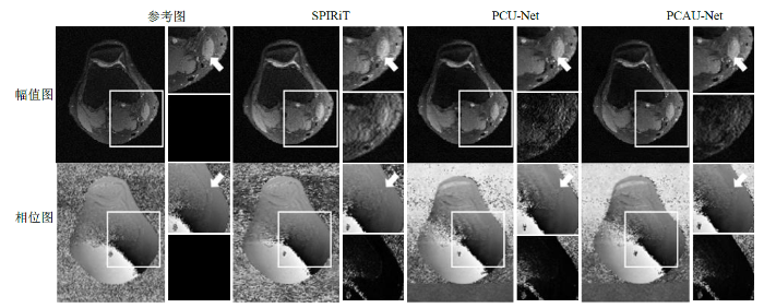
图6
基于随机采样,R = 5时,多通道的幅值和相位的重建图(每幅图左侧)、局部放大图(每幅图右上)、局部误差放大图(每幅图右下)
Fig. 6
Reconstructed amplitude and phase maps (left in each figure), and their local enlarged maps (upper right in each figure) and local error enlarged maps (lower right in each figure) of the multi-channels based on random sampling with R = 5
3.3.2 不同网络架构多通道数据重建图像的客观量化指标对比
表4是基于随机采样,不同加速因子下的不同算法重建的100张测试图像的平均定量分析结果.在R=2.5时,SPIRiT算法重建图像的质量比起PCU-Net和PCAU-Net网络较低,但是差距不大,并且SPIRiT的SSIM和PSNR值与PCU-Net非常接近.在R=5.0时,SPIRiT的SSIM值降到了0.905 1,而PCU-Net和PCAU-Net的SSIM值保持在0.95以上;SPIRiT的PSNR值降到了26.614 3,而PCU-Net和PCAU-Net的SSIM值保持在31以上,由此可见SPIRiT算法在加速因子过高的情况下,重建图像质量也会明显下降.总体上来看,虽然在加速因子R=4.0和5.0时,PCU-Net网络重建的图像的TRE值低于PCAU-Net网络,并且在加速因子R = 4.6时,PCU-Net网络的SSIM值也高于PCAU-Net网络,而在其余加速因子的情况下,PCAU-Net重建出来的图像的PSNR、SSIM值要高于PCU-Net和SPIRiT算法,并且TRE值更低.结合表2来看,PCAU-Net网络无论在规则还是随机采样模式下,图像的重建质量要更高.
表4 基于随机采样,在不同加速因子下,不同算法重建图像的定量指标的平均值
Table 4
| 量化指标 | SPIRiT | PCU-Net | PCAU-Net | ||||
|---|---|---|---|---|---|---|---|
| TRE | R = 2.5 | 1.10×10⁻³ | 7.8081×10⁻⁴ | 7.7575×10⁻⁴ | |||
| R = 3.3 | 1.10×10⁻³ | 8.3336×10⁻⁴ | 8.1667×10⁻⁴ | ||||
| R = 4.0 | 1.50×10⁻³ | 8.7133×10⁻⁴ | 8.9446×10⁻⁴ | ||||
| R = 4.6 | 1.40×10⁻³ | 9.4146×10⁻⁴ | 9.0757×10⁻⁴ | ||||
| R = 5.0 | 1.90×10⁻³ | 9.8781×10⁻⁴ | 9.9610×10⁻⁴ | ||||
| SSIM | R = 2.5 | 0.9629 | 0.9656 | 0.9727 | |||
| R = 3.3 | 0.9588 | 0.9642 | 0.9694 | ||||
| R = 4.0 | 0.9327 | 0.9632 | 0.9720 | ||||
| R = 4.6 | 0.9419 | 0.9596 | 0.9593 | ||||
| R = 5.0 | 0.9051 | 0.9536 | 0.9660 | ||||
| PSNR | R = 2.5 | 33.2773 | 33.2802 | 33.9417 | |||
| R = 3.3 | 32.7259 | 32.9076 | 33.5339 | ||||
| R = 4.0 | 29.0483 | 32.7743 | 33.5606 | ||||
| R = 4.6 | 27.8330 | 32.3175 | 32.4758 | ||||
| R = 5.0 | 26.6143 | 31.8950 | 32.1532 | ||||
注:黑体表示最优指标数据.
3.4 不同算法重建时间和参数量对比
传统GRAPPA并行成像算法的平均重建时间为0.91 s,而PCU-Net和PCAU-Net先进行网络训练,然后利用训练好的网络参数进行图像重建.PCU-Net的训练时间为4.05 h,重建时间为0.20 s;PCAU-Net的训练时间为3.60 h,重建时间为0.17 s.可以看出PCAU-Net的训练时间比PCU-Net短,重建速度快.虽然这两种算法需要预先进行网络训练才能进行图像重建,但是当网络训练完成后,就可以对图像进行快速批量重建.
在相同数据集、相同层数下,本文对比了PU-Net、PCU-Net和PCAU-Net的参数量.其中,PU-Net的卷积、批标准化和激活函数都是基于实数运算,8通道的复数数据的实部和虚部作为16通道的实数数据输入PU-Net.经过实验后得出,PU-Net网络的参数量最少,为16 272 kB;加入复数运算后的PCU-Net增多为26 274 kB;而PCAU-Net的参数量为25 359 kB,少于PCU-Net的参数量.
4 结论
本文提出的基于PCAU-Net的快速多通道MRI方法是一种端到端的深度学习方法,在神经网络模型训练好之后,可以进行批量图像重建且重建速度较快,可以满足临床辅助诊断成像的需求.该方法的重建效果优于经典并行成像算法GRAPPA和SPIRiT算法,且在高加速因子情况下,该方法仍能取得高质量的重建图像;相比于PCU-Net方法,PCAU-Net进一步减少了模型参数、缩短了训练时间.
利益冲突
无
参考文献
Medical progress: Magnetic resonance imaging
[J].DOI:10.1056/NEJM199303183281109 URL [本文引用: 1]
Introduction to functional magnetic resonance imaging: principles and techniques
[M].
Magnetic resonance imaging
[J].
Parallel magnetic resonance imaging
[J].
DOI:10.1088/0031-9155/52/7/R01
PMID:17374908
[本文引用: 1]

Parallel imaging has been the single biggest innovation in magnetic resonance imaging in the last decade. The use of multiple receiver coils to augment the time consuming Fourier encoding has reduced acquisition times significantly. This increase in speed comes at a time when other approaches to acquisition time reduction were reaching engineering and human limits. A brief summary of spatial encoding in MRI is followed by an introduction to the problem parallel imaging is designed to solve. There are a large number of parallel reconstruction algorithms; this article reviews a cross-section, SENSE, SMASH, g-SMASH and GRAPPA, selected to demonstrate the different approaches. Theoretical (the g-factor) and practical (coil design) limits to acquisition speed are reviewed. The practical implementation of parallel imaging is also discussed, in particular coil calibration. How to recognize potential failure modes and their associated artefacts are shown. Well-established applications including angiography, cardiac imaging and applications using echo planar imaging are reviewed and we discuss what makes a good application for parallel imaging. Finally, active research areas where parallel imaging is being used to improve data quality by repairing artefacted images are also reviewed.
An algorithm for NMR imaging reconstruction based on multiple RF receiver coils
[J].DOI:10.1016/0022-2364(87)90348-9 URL [本文引用: 1]
Fast MRI data acquisition using multiple detectors
[J].We present a novel imaging procedure using multiple receiver coils. This circumvents the sequential acquisition of signals required by conventional imaging strategies. The advantage of this technique over existing subsecond imaging techniques is that (a) contrast can be maintained and (b) there is no magnetic field gradient switching involved.
Generalized autocalibrating partially parallel acquisitions (GRAPPA)
[J].
DOI:10.1002/mrm.10171
PMID:12111967
[本文引用: 1]
In this study, a novel partially parallel acquisition (PPA) method is presented which can be used to accelerate image acquisition using an RF coil array for spatial encoding. This technique, GeneRalized Autocalibrating Partially Parallel Acquisitions (GRAPPA) is an extension of both the PILS and VD-AUTO-SMASH reconstruction techniques. As in those previous methods, a detailed, highly accurate RF field map is not needed prior to reconstruction in GRAPPA. This information is obtained from several k-space lines which are acquired in addition to the normal image acquisition. As in PILS, the GRAPPA reconstruction algorithm provides unaliased images from each component coil prior to image combination. This results in even higher SNR and better image quality since the steps of image reconstruction and image combination are performed in separate steps. After introducing the GRAPPA technique, primary focus is given to issues related to the practical implementation of GRAPPA, including the reconstruction algorithm as well as analysis of SNR in the resulting images. Finally, in vivo GRAPPA images are shown which demonstrate the utility of the technique.Copyright 2002 Wiley-Liss, Inc.
SENSE: sensitivity encoding for fast MRI
[J].New theoretical and practical concepts are presented for considerably enhancing the performance of magnetic resonance imaging (MRI) by means of arrays of multiple receiver coils. Sensitivity encoding (SENSE) is based on the fact that receiver sensitivity generally has an encoding effect complementary to Fourier preparation by linear field gradients. Thus, by using multiple receiver coils in parallel scan time in Fourier imaging can be considerably reduced. The problem of image reconstruction from sensitivity encoded data is formulated in a general fashion and solved for arbitrary coil configurations and k-space sampling patterns. Special attention is given to the currently most practical case, namely, sampling a common Cartesian grid with reduced density. For this case the feasibility of the proposed methods was verified both in vitro and in vivo. Scan time was reduced to one-half using a two-coil array in brain imaging. With an array of five coils double-oblique heart images were obtained in one-third of conventional scan time. Magn Reson Med 42:952-962, 1999.Copyright 1999 Wiley-Liss, Inc.
SPIRiT: Iterative self-consistent parallel imaging reconstruction from arbitrary k-space
[J].DOI:10.1002/mrm.22428 URL [本文引用: 2]
Deep learning: Methods and applications
[J].
Deep learning
[J].DOI:10.1038/nature14539 URL [本文引用: 1]
U-net: Convolutional networks for biomedical image segmentation
[C]//
Accelerating magnetic resonance imaging via deep learning
[C]//
Data consistency networks for (calibration-less) accelerated parallel MR image reconstruction
[EB/OL].
Σ-net: Ensembled iterative deep neural networks for accelerated parallel MR image reconstruction
[EB/OL].
GrappaNet: Combining parallel imaging with deep learning for multi-coil MRI reconstruction
[C]//
Deep residual learning for accelerated MRI using magnitude and phase networks
[J].
DOI:10.1109/TBME.2018.2821699
PMID:29993390
[本文引用: 2]
Accelerated magnetic resonance (MR) image acquisition with compressed sensing (CS) and parallel imaging is a powerful method to reduce MR imaging scan time. However, many reconstruction algorithms have high computational costs. To address this, we investigate deep residual learning networks to remove aliasing artifacts from artifact corrupted images.The deep residual learning networks are composed of magnitude and phase networks that are separately trained. If both phase and magnitude information are available, the proposed algorithm can work as an iterative k-space interpolation algorithm using framelet representation. When only magnitude data are available, the proposed approach works as an image domain postprocessing algorithm.Even with strong coherent aliasing artifacts, the proposed network successfully learned and removed the aliasing artifacts, whereas current parallel and CS reconstruction methods were unable to remove these artifacts.Comparisons using single and multiple coil acquisition show that the proposed residual network provides good reconstruction results with orders of magnitude faster computational time than existing CS methods.The proposed deep learning framework may have a great potential for accelerated MR reconstruction by generating accurate results immediately.
A Deep recursive cascaded convolutional network for parallel MRI
[J].
基于深度递归级联卷积神经网络的并行磁共振成像方法
[J].
Deep complex networks
[EB/OL].
Complex fully convolutional neural networks for MR image reconstruction
[C]// International Workshop on Machine Learning for Medical Image Reconstruction.
Laplacian pyramid-based complex neural network learning for fast MR imaging
[C]//
DeepcomplexMRI: Exploiting deep residual network for fast parallel MR imaging with complex convolution
[J].
DOI:S0730-725X(19)30533-8
PMID:32045635
[本文引用: 1]
This paper proposes a multi-channel image reconstruction method, named DeepcomplexMRI, to accelerate parallel MR imaging with residual complex convolutional neural network. Different from most existing works which rely on the utilization of the coil sensitivities or prior information of predefined transforms, DeepcomplexMRI takes advantage of the availability of a large number of existing multi-channel groudtruth images and uses them as target data to train the deep residual convolutional neural network offline. In particular, a complex convolutional network is proposed to take into account the correlation between the real and imaginary parts of MR images. In addition, the k-space data consistency is further enforced repeatedly in between layers of the network. The evaluations on in vivo datasets show that the proposed method has the capability to recover the desired multi-channel images. Its comparison with state-of-the-art methods also demonstrates that the proposed method can reconstruct the desired MR images more accurately.Copyright © 2020 Elsevier Inc. All rights reserved.
3D MRI brain tumor segmentation using autoencoder regulari-zation
[C]//
Going deeper with convolutions
[C]//
Deep residual learning for image recognition
[C]//
Image quality assessment: from error visibility to structural similarity
[J].
DOI:10.1109/tip.2003.819861
PMID:15376593
[本文引用: 1]
Objective methods for assessing perceptual image quality traditionally attempted to quantify the visibility of errors (differences) between a distorted image and a reference image using a variety of known properties of the human visual system. Under the assumption that human visual perception is highly adapted for extracting structural information from a scene, we introduce an alternative complementary framework for quality assessment based on the degradation of structural information. As a specific example of this concept, we develop a Structural Similarity Index and demonstrate its promise through a set of intuitive examples, as well as comparison to both subjective ratings and state-of-the-art objective methods on a database of images compressed with JPEG and JPEG2000.
Coil compression for accelerated imaging with Cartesian sampling
[J].
DOI:10.1002/mrm.24267
PMID:22488589
[本文引用: 1]
MRI using receiver arrays with many coil elements can provide high signal-to-noise ratio and increase parallel imaging acceleration. At the same time, the growing number of elements results in larger datasets and more computation in the reconstruction. This is of particular concern in 3D acquisitions and in iterative reconstructions. Coil compression algorithms are effective in mitigating this problem by compressing data from many channels into fewer virtual coils. In Cartesian sampling there often are fully sampled k-space dimensions. In this work, a new coil compression technique for Cartesian sampling is presented that exploits the spatially varying coil sensitivities in these nonsubsampled dimensions for better compression and computation reduction. Instead of directly compressing in k-space, coil compression is performed separately for each spatial location along the fully sampled directions, followed by an additional alignment process that guarantees the smoothness of the virtual coil sensitivities. This important step provides compatibility with autocalibrating parallel imaging techniques. Its performance is not susceptible to artifacts caused by a tight imaging field-of-view. High quality compression of in vivo 3D data from a 32 channel pediatric coil into six virtual coils is demonstrated.Copyright © 2012 Wiley Periodicals, Inc.
