

1 引言
近年来, 不可压缩流与多孔介质流之间的耦合问题受到人们的广泛关注. 该耦合问题能够有效地模拟地表水与地下水之间的运移问题, 石油开采问题, 工业中与流体过滤有关的问题以及生物流体力学中的血液循环问题等. Navier-Stokes/Darcy 模型和 Stokes/Darcy 模型是研究该耦合问题的重要模型, 研究者已经针对这两个模型进行了深入的研究. 本文重点讨论 Stokes/Darcy 模型。
目前, 针对定常 Stokes/Darcy 模型的研究已经相对成熟, 其数值方法包括有限元法[1⇓⇓⇓-5], 间断伽辽金法[6⇓-8], 界面松弛法[9-10], 拉格朗日乘子法[11-12], 区域分解法[13⇓-15], 两重网格或多重网格法[16⇓⇓-19]等. 现在, 学者们越来越重视非定常 Stokes/Darcy 模型的研究, 并通过不同的方法获得其时间半离散格式的相关结论. 如整体相同时间步长方法[20⇓-22], 不同区域不同时间步长方法[23⇓⇓-26]. 然而, 现存的方法仍然存在一些不足. 例如, 某类数值方法需要消耗大量的计算时间才能得到相对较高的数值精度; 某类算法需要对时间步长给予特定的限制条件其稳定性和误差估计才能得到证明; 某类算法的稳定性需要增加一个稳定化项才能得到证明. 因此, 研究更高效, 适应性更强的算法是十分必要的.
多步法是求解常微分方程初值问题的基本数值解法. 多步法的主要思想是保留和使用前面多步数值来预测当前时刻数值使算法尽可能获得较高精度. 本文的研究基于一阶线性多步法的
本文的其余部分组织如下: 第 2 节介绍具有 Beavers-Joseph Saffman (BJS) 界面条件的 Stokes/Darcy 模型, 并给出其弱形式; 第 3 节提出耦合和解耦的线性多步法加 time filter 算法并分析其稳定性; 第 4 节分析耦合和解耦算法的误差估计; 第 5 节利用数值试验进一步佐证理论分析的结果.
2 Stokes/Darcy 模型和弱形式
在有界光滑区域
图 1

本文研究由 Stokes 方程和 Darcy 方程组成的 Stokes/Darcy 模型. 设
其中
分别是应力张量和应变张量,
多孔介质区域
其中, 第一个方程是饱和流动模型,
将方程(2.4)代入方程(2.3)可得 Darcy 方程: 求测压水头
下面考虑 Stokes/Darcy 模型满足以下初值条件
以及齐次 Dirichlet 边界条件
交界面条件是 Stokes/Darcy 模型的重要组成部分, 包括质量守恒条件, 法向力的平衡条件和 Beavers-Joseph-Saffman(BJS) 条件. 具体表示如下: 在
其中
首先定义 Hilbert 空间
区域
用
对函数
其次, 非定常Stokes/Darcy 耦合模型(2.1)-(2.10)式的弱形式描述如下: 对于
其中
双线性形式
下面给出Poincar
定常的耦合Stokes/Darcy 模型的适定性已被证明. 这里, 假定在非稳态的情况下也同样成立. 本文主要研究其数值解.
3 数值算法和稳定性
对任意给定的小参数
并定义
定义线性投影算子(见文献[31]):
假设
Inverse 不等式: 存在常数
理论分析时将用到下面两个引理.
另外,
这里引入相关的记号
本节其余部分将给出非定常 Stokes/Darcy 模型耦合和解耦的线性多步法加 time filter 算法以及其稳定性. 将时间段
3.1 耦合算法及其稳定性
耦合的线性多步法加 time filter 算法描述如下.
给定
通过 time filter 算法更新线性多步法的解
下面给出耦合的线性多步法加 time filter 算法的稳定性分析.
其中
将上述两式代入 (3.7) 式,
假设
其次, 利用双线性形式
由无散度特性可知, 左边第三项等于 0. 最后, 根据 Young 不等式和 Cauchy Schwarz 不等式, 有
结合 (3.10)-(3.12) 式, 并将 (3.9) 式从
由于
因此
从而得到耦合算法的稳定性结论.证毕.
3.2 解耦算法及其稳定性
解耦的线性多步法加 time filter 算法表述如下.
给定
给定
通过 time filter 算法更新线性多步法的解
下面给出解耦的线性多步法加 time filter 算法的稳定性分析.
其中
将上述三式分别代入 (3.13) 和 (3.14) 式后相加,
假设
这里主要分析交界面项. 借助引理 3.2, 并代入
其中, 最后一个不等式是在选择合适的常量
结合 (3.17)-(3.23) 式, 并将 (3.16) 式从
由于
以及
因此
结合离散的 Gronwall 引理可得解耦算法的稳定性结论. 证毕.
4 误差估计
本节将证明耦合和解耦算法的误差估计. 记算法的精确解为
显然地, 下述关系式成立
需注意
假设所求解满足下述正则性条件
外力项
4.1 耦合算法的误差估计
假设
首先, 借助引理 3.1, 有
利用双线性形式
由无散度特性可知, 左边第三项的结果为 0.
其次, 利用积分型余项的泰勒展开式,有
代入并整理得
再结合 Cauchy-Schwarz 不等式,有
可以得到
类似地, 借助积分型余项的泰勒展开式,有
代入并整理得
从而
类似地, 根据积分型余项的泰勒展开式,有
代入并整理得
从而
最后, 结合 (4.5)-(4.8) 式, 将 (4.4) 式从
由三角不等式可得耦合算法误差估计的结论. 证毕.
4.2 解耦算法的误差估计
假设
下面主要分析交界面项. 交界面项可以被分解为
由线性性质可知, 上式中前四项之和等于
其中, 最后一个不等式是在选择合适的常量
利用带有积分型余项的泰勒展开式,有
代入并整理得
类似地, 根据带有积分型余项的泰勒展开式,有
可以得到
利用引理 3.2 并代入
其中, 第二个不等式是在选择合适的常量
综上, 交界面项可化简为
结合 (4.10)-(4.23) 式, 将 (4.9) 式从
由三角不等式可得解耦算法误差估计的结论.证毕.
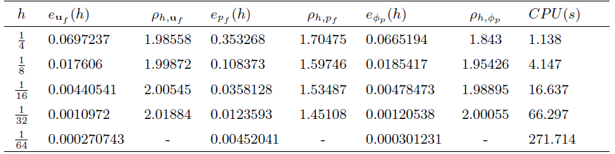
5 数值实验
这一节将进行3个数值实验. 第1个实验对耦合和解耦算法的有效性进行模拟. 第2个实验说明算法的收敛阶由一阶提高到二阶, 并通过对比体现出解耦算法的高效性. 第3个实验将耦合和解耦的向后欧拉方法和取不同
图 2

图 3

图 4

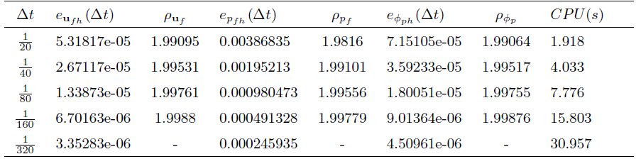

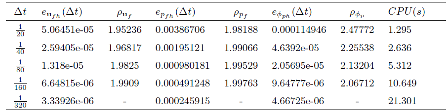
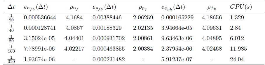


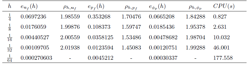
首先, 利用与文献[31] 中相同的方法, 通过固定网格尺寸
其中
其次, 在固定时间步长
图 5 分别给出了向后欧拉方法和
图 5
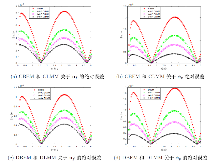
图 6

参考文献
Approximation of coupled Stokes-Darcy flow in an axisymmetric domain
DOI:10.1016/j.cma.2013.02.004 URL [本文引用: 1]
On the solution of coupled Stokes/Darcy model with Beavers-Joseph interface condition
DOI:10.1016/j.camwa.2018.09.011 URL [本文引用: 1]
Finite element approximations for Stokes-Darcy flow with Beavers-Joseph interface conditions
DOI:10.1137/080731542 URL [本文引用: 1]
A strongly conservative finite element method for the coupling of Stokes and Darcy flow
DOI:10.1016/j.jcp.2010.04.021 URL [本文引用: 1]
Finite element methods for incompressible viscous flow
Discontinuous Galerkin and mimetic finite difference methods for coupled Stokes-Darcy flows on polygonal and polyhedral grids
DOI:10.1007/s00211-013-0563-3 URL [本文引用: 1]
Weak Galerkin method for the coupled Darcy-Stokes flow
DOI:10.1093/imanum/drv012 URL [本文引用: 1]
DG approximation of coupled Navier-Stokes and Darcy equations by Beaver-Joseph-Saffman interface condition
DOI:10.1137/070686081 URL [本文引用: 1]
An agent-based netcentric framework for multidisciplinary problem solving environments (MPSE)
DOI:10.33545/26633582 URL [本文引用: 1]
Solving composite problems with interface relaxation
DOI:10.1137/S1064827597321180 URL [本文引用: 1]
A residual-based a posteriori error estimator for a fully-mixed formulation of the Stokes-Darcy coupled problem
DOI:10.1016/j.cma.2011.02.009 URL [本文引用: 1]
Coupling fluid flow with porous media flow
DOI:10.1137/S0036142901392766 URL [本文引用: 1]
A domain decomposition method for the steady-state Navier-Stokes-Darcy model with Beavers-Joseph interface condition
DOI:10.1137/140965776 URL [本文引用: 1]
Robin-Robin domain decomposition methods for the steady Stokes-Darcy model with Beaver-Joseph interface condition
DOI:10.1007/s00211-011-0361-8 URL [本文引用: 1]
A parallel Robin-Robin domain decomposition method for the Stokes-Darcy system
DOI:10.1137/080740556 URL [本文引用: 1]
Optimal error estimates of a decoupled scheme based on two-grid finite element for mixed Stokes-Darcy model
DOI:10.1016/j.aml.2016.01.007 URL [本文引用: 1]
Optimal error estimates of a decoupled scheme based on two-grid finite element for mixed Navier-Stokes/Darcy model
DOI:10.1016/S0252-9602(18)30819-1 URL [本文引用: 1]
A multi-grid technique for coupling fluid flow with porous media flow
DOI:10.1016/j.camwa.2018.03.010 URL [本文引用: 1]
A two-grid decoupling method for the mixed Stokes-Darcy model
DOI:10.1016/j.cam.2014.08.008 URL [本文引用: 1]
Coupled Stokes-Darcy model with Beavers-Joseph interface boundary condition
DOI:10.4310/CMS.2010.v8.n1.a2 URL [本文引用: 1]
Parallel, non-iterative, multi-physics domain decomposition methods for time-dependent Stokes-Darcy systems
DOI:10.1090/mcom/2014-83-288 URL [本文引用: 1]
Finite element approximation for time-dependent Stokes-Darcy flow with Beavers-Joseph interface boundary condition
DOI:10.1137/080731542 URL [本文引用: 1]
A second-order partitioned method with different subdomain time steps for the evolutionary Stokes-Darcy system
DOI:10.1002/mma.v41.5 URL [本文引用: 1]
Long time stability of four methods for splitting the evolutionary Stokes-Darcy problem into Stokes and Darcy subproblems
DOI:10.1016/j.cam.2012.02.019 URL [本文引用: 1]
Analysis of long time stability and errors of two partitioned methods for uncoupling evolutionary groundwater-surface water flows
DOI:10.1137/110834494 URL [本文引用: 1]
A decoupling method with different subdomain time steps for the nonstationary Stokes-Darcy model
DOI:10.1002/num.v29.2 URL [本文引用: 1]
Time filters increase accuracy of the fully implicit method
Adaptive partitioned methods for the time-accurate approximation of the evolutionary Stokes-Darcy system
DOI:10.1016/j.cma.2020.112923 URL [本文引用: 1]
The time filter for the non-stationary coupled Stokes/Darcy model
DOI:10.1016/j.apnum.2019.07.015
[本文引用: 1]

In this paper, we consider the effect of adding a simple time filter to the Backward Euler scheme for the non-stationary coupled Stokes/Darcy model. The method is modular and requires only one additional line of code to be added, which improves the accuracy of the Backward Euler scheme from first to second order. We verify this conclusion from both theoretical analysis and numerical experiments. Finally, we propose that the BDF2 scheme can be improved to the third order if the time filter is added, which is demonstrated by numerical experiments. (C) 2019 IMACS. Published by Elsevier B.V.
Decoupled schemes for a non-stationary mixed Stokes-Darcy model
DOI:10.1090/S0025-5718-09-02302-3 URL [本文引用: 3]
A variable time step time filter algorithm for the geothermal system
A parallel Robin-Robin domain decomposition method based on modified characteristic FEMs for the time-dependent dual-porosity-Navier-Stokes model with the Beavers-Joseph interface condition
DOI:10.1007/s10915-021-01681-y
An efficient ensemble algorithm for numerical approximation of stochastic Stokes-Darcy equations
DOI:10.1016/j.cma.2018.08.020
[本文引用: 1]
We propose and analyze an efficient ensemble algorithm for fast computation of multiple realizations of the stochastic Stokes-Darcy model with a random hydraulic conductivity tensor. The algorithm results in a common coefficient matrix for all realizations at each time step making solving the linear systems much less expensive while maintaining comparable accuracy to traditional methods that compute each realization separately. Moreover, it decouples the Stokes-Darcy system into two smaller sub-physics problems, which reduces the size of the linear systems and allows parallel computation of the two sub-physics problems. We prove the ensemble method is long time stable and first-order in time convergent under a time-step condition and two parameter conditions. Numerical examples are presented to support the theoretical results and illustrate the application of the algorithm. (C) 2018 Elsevier B.V.
A second-order artificial compression method for the evolutionary Stokes-Darcy system
DOI:10.1007/s11075-019-00791-x [本文引用: 1]
Error estimates of second-order decoupled scheme for the evolutionary Stokes-Darcy system
