


引言
肝脏的磁共振$R_{2}^{*}$参数图像能够反映肝脏内铁沉积的空间分布[5]. 传统的$R_{2}^{*}$参数图像重建技术将不同回波时间(TE)采集的$T_{2}^{*}$加权图像逐像素拟合到单指数物理衰减模型,从而得到$R_{2}^{*}$参数图像. 但是,磁共振采集得到的铁沉积肝脏$T_{2}^{*}$加权图像通常信噪比较低,幅值图像中的噪声通常可以用莱斯分布或者非中心卡方分布来描述[6]. 噪声的存在会影响$R_{2}^{*}$定量的准确性. 为了提高$R_{2}^{*}$参数估计的准确性,需要校正噪声对$R_{2}^{*}$量化造成的偏差. 基于一阶矩噪声校正模型(M1NCM)和基于二阶矩噪声校正模型(M2NCM)的两种参数拟合算法分别通过将测量信号拟合到一阶矩和二阶矩噪声校正模型来计算$R_{2}^{*}$值,显著地提高了$R_{2}^{*}$量化的准确性[7]. 但是,上述两种方法采取的均为逐像素拟合的方式,重建得到的$R_{2}^{*}$参数图像依旧会受到噪声的影响. 基于自适应邻域正则化的算法(PCANR)[8]将图像噪声抑制和曲线拟合纳入到一个统一约束框架中,显著地降低了噪声的影响,同时能够很好地保留$R_{2}^{*}$参数图像中的细节结构. 尽管PCANR算法取得了很好的$R_{2}^{*}$参数图像重建效果,但是,参数图像重建过程比较耗时,不利于临床的推广应用.
最近,深度学习网络被广泛应用于磁共振参数图像重建中[9]. 深度学习网络通过训练数据学习输入与输出之间的非线性关系,直接将输入不同对比度的磁共振加权图像映射到参数图像. 基于深度学习网络的参数图像重建算法重建速度快,参数图像质量高,能够很好地抑制噪声的影响. 但是,这些网络通常需要真实的或者高质量的参数图像作为目标进行训练. 考虑到图像采集和处理的时间,高质量参数图像的获得通常比较困难. 因此,本文提出了一种模型引导的自监督深度学习网络(UNet-TVp)用于铁沉积肝脏磁共振$R_{2}^{*}$参数图像重建方法,通过噪声校正模型和改进的全变分(Total Variation,TV)模型对深度学习网络的训练进行引导,从而不需要真实的或者高质量的$R_{2}^{*}$参数图像作为标签来进行训练,只需要临床采集得到的带有噪声的肝脏$T_{2}^{*}$加权图像进行自监督训练. 该方法可以对噪声造成的$R_{2}^{*}$参数估计偏差进行校正,有效抑制噪声的影响,快速重建得到高质量的铁沉积肝脏的$R_{2}^{*}$参数图像.
1 材料和方法
1.1 模型引导的自监督深度学习网络
1.1.1 网络的构建
本文提出的模型引导的自监督深度学习网络UNet-TVp的总体框架如图1所示. 网络的输入为不同TE采集得到的肝脏$T_{2}^{*}$加权图像$X=({{S}_{1}},{{S}_{2}},\cdots,{{S}_{N}})$,其中,N为$T_{2}^{*}$加权图像采集过程中使用的回波数量. 应用卷积神经网络U从输入的$T_{2}^{*}$加权图像中估计得到对应的参数图像$P=({{S}_{0}},R_{2}^{*})$,即$P=U(X)$,其中,${{S}_{0}}$为TE = 0时的$T_{2}^{*}$加权信号图像,$R_{2}^{*}$为所要估计的磁共振$R_{2}^{*}$参数图像. 估计得到的参数图像P可以通过信号生成模型M重新合成$T_{2}^{*}$加权图像${{X}^{*}}=(S_{1}^{*},S_{2}^{*},\cdots,S_{N}^{*})$,即${{S}^{*}}=M(P)$.
图1
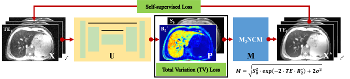
通常,在噪声的影响下,使用简单的单指数物理衰减模型作为信号生成模型M会引起参数估计的偏差.
为了校正噪声引起的参数估计偏差,我们使用了M2NCM[7]作为信号生成模型M,可以表示为:
其中,$\text{T}{{\text{E}}_{n}}$为第n个TE,$n\in (1,2,\cdots,N)$,σ为肝脏$T_{2}^{*}$加权图像中的噪声标准差,其可以通过图像背景信号估计得到,计算方法为背景区域手动选择的感兴趣区域(ROI)内的信号平均值乘以0.8[8]. 本文使用的卷积神经网络U基于传统的2D U-Net结构[10]构建而成,如图2所示. U-Net网络已经被广泛应用于磁共振参数重建研究中[11,12]. 网络的输入为12通道的二维图像,其中,不同通道分别对应不同TE采集的肝脏$T_{2}^{*}$加权图像. 网络的输出为2通道,分别对应于${{S}_{0}}$和$R_{2}^{*}$参数图像. 本文使用的U-Net网络具有对称结构,包括一个编码网络和一个解码网络. 编码网络从输入图像中提取空间不变的图像特征,而解码网络通过不同尺度的反卷积来恢复图像的细节. 编码网络和解码网络之间的跳跃连接用来融合特征. U-Net这种多尺度的结构能够有效利用图像中的全局信息.
图2
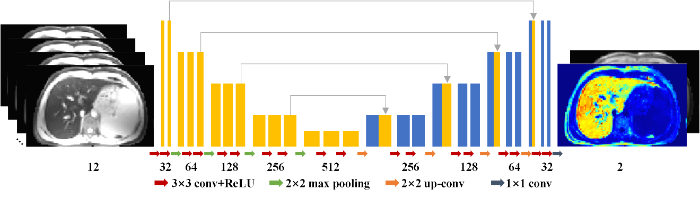
图2
卷积神经网络的结构. 网络的输入为不同TE时间采集得到的12幅肝脏$T_{2}^{*}$加权图像,输出为2幅参数图像,分别对应着${{S}_{0}}$和$R_{2}^{*}$参数图像
Fig. 2
The architecture of the convolutional neural network used in the proposed method. The inputs of the network are 12$T_{2}^{*}$-weighted images acquired at different TEs, and the outputs are 2 parameter maps corresponding to${{S}_{0}}$and$R_{2}^{*}$maps, respectively
1.1.2 损失函数
为了实现网络的自监督训练,本文提出的方法UNet-TVp使用了一种新型损失函数,可以表示为:
其中,${{L}_{\text{self}}}$为自监督损失(Self-supervised Loss),${{L}_{\text{TVp}}}$为一种改进的TV损失(Total Variation Loss),权重参数λ用来平衡两种损失之间的影响. 自监督损失${{L}_{\text{self}}}$计算合成的$T_{2}^{*}$加权图像${{X}^{*}}$和输入X之间的均方误差,可以表示为:
其中,M为单幅$T_{2}^{*}$加权图像中的像素数目. 传统的TV损失(${{L}_{\text{TV}}}$)计算重建的参数图像的TV值[13],可以表示为:
其中,a为阈值参数. 相较于传统的TV模型,改进的TV模型减弱了对于梯度值大于a的图像区域的约束. 因此,本文提出的方法UNet-TVp使用的${{L}_{\text{TVp}}}$可以表示为:
1.2 实验设计
1.2.1 实验数据集
为了验证本文提出的深度学习网络的$R_{2}^{*}$参数图像重建性能,实验采集了100位患有地中海贫血的病人的肝脏磁共振数据. 本研究已经获得了伦理委员会的批准以及患者的知情同意书. 实验数据是在1.5 T Siemens Sonata磁共振扫描仪上采集的,同时使用一个8通道的阵列线圈. 轴向的肝脏$T_{2}^{*}$加权图像通过2D的多回波梯度回波序列采集,采集参数为:重复时间为200 ms,最小TE为0.93 ms,回波数为12,回波间隔为1.34 ms,翻转角为20˚,层厚为10 mm,采集矩阵为64×128,分辨率为3.125×3.125 mm2. 同时,使用脂肪饱和技术来消除脂肪的影响. 在采集的数据集中随机选取80个作为网络的训练集(其中15个作为验证集用于超参数的调节),剩余的20个作为网络的测试集. 为了将图像中像素值的取值范围转化到大约为0~1的范围内,同时保持不同病人数据中的噪声水平相对大小不变,采集得到的肝脏$T_{2}^{*}$加权图像通过将图像中每个像素值除以整个数据集的像素值的95%分位数进行了标准化处理. 为了增加训练数据的数量,在训练过程中,我们从原始图像中均匀地提取大小为64×64的图像块作为训练的样本,提取区域的移动步长为8,同时使用了数据扩增技术,包括对图像块进行旋转(旋转角度为90˚、180˚和270˚)和翻转操作. 最终,训练数据集中的样本个数为5 760. 网络进行测试时将整幅完整图像作为输入进行$R_{2}^{*}$参数图像的重建.
为了定量地评估不同方法的$R_{2}^{*}$参数图像重建表现,本研究使用测试集中的临床肝脏数据合成了对应的仿真肝脏测试数据. 由临床数据生成的仿真肝脏数据保留了肝脏的组织结构特征,能够较好地模拟临床采集得到的肝脏$T_{2}^{*}$加权图像. 首先,测试集中的临床数据通过PCANR算法产生质量较好的${{S}_{0}}$和$R_{2}^{*}$参数图像. 然后,将生成的${{S}_{0}}$和$R_{2}^{*}$参数图像作为真实参数图像并结合单指数物理模型$S={{S}_{0}}\cdot \exp (-TE*R_{2}^{*})$合成仿真的肝脏$T_{2}^{*}$加权图像,其中,仿真过程使用的TE值和用于采集临床肝脏数据的TE值相同. 最后,在仿真肝脏$T_{2}^{*}$加权图像中加入与临床数据相同水平的莱斯噪声作为最终的仿真肝脏测试数据. 噪声的标准差为7.5(标准化之前),为所有临床数据中噪声标准差的平均值.
1.2.2 实验设置及对比方法
为了验证本文提出方法的$R_{2}^{*}$参数图像重建性能,我们与传统的基于模型的$R_{2}^{*}$参数图像重建算法进行了对比,分别为:基于单指数物理衰减模型的最小二乘拟合(EXP),M2NCM[7],M1NCM[7]以及PCANR算法[8]. 此外,为了验证噪声校正模型[(2)式]引导网络校正偏差的作用以及改进的TV模型[(7)式]的去噪作用,我们将本文提出的方法(UNet-TVp)与仅使用单指数物理衰减模型[(1)式]引导的网络(UNet-EXP)[12]、仅使用噪声校正模型引导的网络(UNet-M2)以及使用噪声校正模型和传统的TV模型[(5)式]共同引导的网络(UNet-TV)进行了对比. 其中,UNet-TV中参数λ根据经验设置为0.001,UNet-TVp中阈值参数a根据文献[18]设置为0.1,参数λ设置为0.003. 为了探究不同大小的权重参数λ对UNet-TVp网络表现的影响,我们在保持其它参数不变的情况下,训练了λ = 0、0.002、0.003和0.004不同条件下的UNet-TVp网络. 上述所有深度学习网络除了使用的损失函数不同外,都使用了相同的卷积神经网络、训练数据以及训练参数设置.
本文中所有网络都应用TensorFlow深度学习框架来实现网络的训练和测试,使用NVIDIA GeForce TITAN X Pascal图像处理单元进行训练. 卷积神经网络的权重参数使用MSRA[19]初始化方法进行初始化,训练过程中使用Adam算法更新网络参数,其初始学习率为0.000 5并随着训练的进行逐渐减小. 批处理的大小设置为32,训练轮数为200.
1.2.3 评估标准及统计分析
其中,$\hat{R}_{2}^{*}$和$R_{2}^{*}$分别为重建图像和参考图像的$R_{2}^{*}$值,$||\cdot |{{|}_{\text{2,ROI}}}$计算ROI内的值的${{l}_{2}}$范数. SSIM对图像的对比度、亮度和结构信息保持进行评估,可以表示为:
其中,${{\mu }_{x}}$和${{\mu }_{y}}$分别为参考图像和重建图像中$R_{2}^{*}$值的均值,${{\sigma }_{x}}$和${{\sigma }_{y}}$分别为参考图像和重建图像中$R_{2}^{*}$值的标准差,${{\sigma }_{xy}}$为参考图像和重建图像中$R_{2}^{*}$值的协方差,${{c}_{1}}={{({{k}_{1}}L)}^{2}}$,${{c}_{2}}={{({{k}_{2}}L)}^{2}}$,其中${{k}_{1}}=0.01$,${{k}_{2}}=0.03$,L为图像的取值范围.SSIM的值也是在感兴趣区域中计算的. 感兴趣区域为通过手工勾画的肝脏区域. 本文的评价指标是通过Python中的scikit-image工具包[22]来实现的. 本文采用常用的SciPy工具包进行统计分析,采用威氏符号秩次检验(Wilcoxon signed-rank test)对不同方法之间定量评估指标差异的显著性进行判断(显著水平P<0.05表示差异具有统计学意义).
2 结果
2.1 仿真肝脏数据结果
图3显示了使用不同大小的权重参数λ训练的UNet-TVp网络重建得到的$R_{2}^{*}$参数图像. 当参数λ设置为0时,图像中的噪声无法得到抑制. 随着λ的增大,$R_{2}^{*}$参数图像越来越平滑,参数图像的误差也逐渐变小. 但是,当权重参数λ设置过大时(λ= 0.004)会产生过平滑的效应,造成$R_{2}^{*}$估计的误差,如图中白色箭头所指的区域所示. 相较于λ= 0、0.002和0.004,在λ= 0.003的情况下,UNet-TVp得到$R_{2}^{*}$参数图像与真实参数图像最为接近,误差也最小. 因此,在后面的实验中选择λ= 0.003作为UNet-TVp的默认参数.
图3
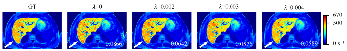
图3
不同大小的权重参数λ情况下训练的UNet-TVp网络重建得到的$R_{2}^{*}$参数图像. $R_{2}^{*}$参数图像的NRMSE值标于图像的右下角. 图片右边色条颜色由蓝到红代表着$R_{2}^{*}$值从小到大的变化(GT:真实参数图像)
Fig. 3
$R_{2}^{*}$ maps reconstructed by UNet-TVp with different λ values. The NRMSE values of $R_{2}^{*}$ maps are shown in the bottom right corner of the maps. The change of color in the color bar on the right side of the figure from blue to red represents the $R_{2}^{*}$ value from small to large (GT: ground truth)
表1 不同方法在仿真肝脏测试数据上得到的定量结果(均值±标准差)
Table 1
| Methods | NRMSE | SSIM | Methods | NRMSE | SSIM | |
|---|---|---|---|---|---|---|
| EXP | 0.0616±0.0358 | 0.9571±0.0506 | UNet-EXP | 0.0623±0.0348 | 0.9572±0.0492 | |
| M2NCM | 0.0605±0.0354 | 0.9548±0.0502 | UNet-M2 | 0.0576±0.0286 | 0.9582±0.0466 | |
| M1NCM | 0.0581±0.0325 | 0.9561±0.0494 | UNet-TV | 0.0494±0.0145 | 0.9724±0.0201 | |
| PCANR | 0.0453±0.0122 | 0.9754±0.0182 | UNet-TVp | 0.0438±0.0100 | 0.9796±0.0117 |
图4显示了一例重度铁沉积肝脏仿真测试数据应用不同方法重建得到的$R_{2}^{*}$参数图像. 基于传统的参数图像重建方法,EXP的结果产生了较大的偏差,尤其是肝右叶部分的值在整体上明显小于真实参数图像中的值,肝脏中的$R_{2}^{*}$值明显被低估. 而基于噪声校正模型的参数拟合算法(M2NCM和M1NCM)能够较好的校正偏差,但是M2NCM和M1NCM得到的$R_{2}^{*}$参数图像仍然受到噪声的影响(如白色箭头所指的区域所示). PCANR能在校正偏差的同时得到质量较高的参数图像. 对于基于深度学习网络的重建方法,UNet-EXP的重建结果与EXP一致,同样产生了较大的偏差. 当使用噪声校正模型对网络的训练进行引导时(UNet-M2),偏差得到了校正,但是其重建得到的$R_{2}^{*}$参数图像中仍然存在噪声(如白色箭头指的区域所示).UNet-TV能够校正偏差的同时抑制噪声的影响. 本文提出的UNet-TVp取得了最好的表现,能够很好地校正偏差,抑制$R_{2}^{*}$参数图像中的噪声,同时取得了最低的NRMSE和最高的SSIM指标.
图4

图4
一例重度铁沉积肝脏仿真测试数据应用不同方法重建得到的$R^{*}_{2}$参数图像以及对应的绝对误差图(Difference). $T^{*}_{2}$ w: $T^{*}_{2}$加权图像(TE1 = 0.93 ms,TE2 = 2.27 ms).GT: 真实$S_{0}$和$R^{*}_{2}$参数图像. $R^{*}_{2}$参数图像的SSIM值标于参数图像的右上角,$R^{*}_{2}$参数图像的NRMSE值标于对应的绝对误差图的右上角. 图片右边色条颜色由蓝到红代表着$R^{*}_{2}$值从小到大的变化
Fig. 4
$R^{*}_{2}$maps reconstructed by different methods for one simulated severe iron-loaded liver dataset and corresponding absolute difference maps (Difference) under each $R^{*}_{2}$ map. $T^{*}_{2}$ w: $T^{*}_{2}$-weighted images (TE1 = 0.93 ms, TE2 = 2.27 ms). GT: ground truth of $S_{0}$ and $R^{*}_{2}$ maps. The SSIM of each $R^{*}_{2}$ map is shown in its top right corner, and the NRMSE is shown in the top right corner of the corresponding absolute difference map. The change of color in the color bar on the right side of the figure from blue to red represents the $R^{*}_{2}$ value from small to large
在仿真肝脏测试数据上,不同方法重建得到的$R_{2}^{*}$参数图像的肝实质中的平均$R_{2}^{*}$值与真实$R_{2}^{*}$值的一致性通过Bland-Altman分析来进行评估(图5).当$R_{2}^{*}$值较大时($R_{2}^{*}$> 300 s-1),EXP和UNet-EXP都会产生明显的低估,而基于噪声校正模型的拟合算法(M2NCM和M1NCM)和UNet-M2都能够对偏差进行一定程度的校正.但是,$R_{2}^{*}$> 700 s-1时,M2NCM会产生明显的高估.UNet-M2的表现与M1NCM方法相近,表现出相似的变化趋势.UNet-TV在$R_{2}^{*}$较大时($R_{2}^{*}$> 500 s-1)仍然产生了$R_{2}^{*}$值的低估.UNet-M2(-0.78)、UNet-TVp(-1.37)和PCANR(-1.43)的平均偏差之间没有明显差异,估计得到的平均$R_{2}^{*}$值与真实$R_{2}^{*}$值都有很好的一致性.
图5

图5
仿真肝脏测试数据应用不同方法估计得到的肝实质内(排除了血管结构)的平均$R^{*}_{2}$值与参考值之间的一致性分析. 图中实线代表平均偏差,虚线代
Fig. 5
Bland-Altman analysis for the agreement between the mean $R^{*}_{2}$ values in liver parenchyma (excluding vasculatures) and the reference, and the $R^{*}_{2}$ maps reconstructed from different methods on the simulated testing datasets. The solid lines represent mean differences and the dashed lines indicate 95% confidence intervals
2.2 临床肝脏数据结果
由于临床数据无法获得真实的$R_{2}^{*}$参数图像,而PCANR算法是当前最优的基于模型的肝脏$R_{2}^{*}$参数图像重建算法,所以在临床肝脏测试数据上,本文以PCANR重建得到的$R_{2}^{*}$参数图像为参照,重点研究了不同方法的结果与PCANR算法之间的一致性.不同方法重建得到的$R_{2}^{*}$参数图像的肝实质中的平均$R_{2}^{*}$值与PCANR方法得到的平均$R_{2}^{*}$值的一致性通过Bland-Altman分析进行了评估(图6).与仿真实验结果基本一致,当$R_{2}^{*}$值超过250 s-1时,随着$R_{2}^{*}$的增大,EXP和UNet-EXP估计得到的肝实质平均$R_{2}^{*}$值与PCANR的结果之间差异越来越大. 在$R_{2}^{*}$值大于500 s-1时,UNet-TV估计得到的$R_{2}^{*}$值明显低于PCANR,M2NCM产生了高估,M1NCM、UNet-M2和UNet-TVp得到结果与PCANR的结果有很好的一致性,这与仿真实验的结果也是一致的.
图6
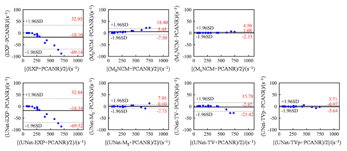
图6
临床肝脏测试数据应用不同方法估计得到的肝实质内(排除了血管结构)的平均$R^{*}_{2}$值与PCANR算法的结果之间的一致性分析. 图中实线代表平均偏差,虚线代
Fig. 6
Bland-Altman analysis for the agreement of the mean $R^{*}_{2}$ values in liver parenchyma (excluding vasculatures) with the reference, and the $R^{*}_{2}$ maps reconstructed from other methods on the clinical testing datasets. The PCANR algorithm was used as the reference method. The solid lines represent mean differences and the dashed lines indicate 95% confidence intervals
图7和图8分别显示了不同方法在中度和重度铁沉积肝脏临床测试数据上重建得到的$R_{2}^{*}$参数图像.与仿真实验一致,EXP和UNet-EXP重建得到的$R_{2}^{*}$参数图像肝脏内的$R_{2}^{*}$值整体上明显小于PCANR的结果,尤其是在重度铁沉积的肝脏数据中.相较于EXP和UNet-EXP算法,M2NCM、M1NCM和UNet-M2重建得到的$R_{2}^{*}$参数图像尽管与PCANR更为接近,参数的相对低估得到了校正,但是仍然会受到噪声的影响.UNet-TV和UNet-TVp都能够抑制噪声的影响,但是UNet-TV在重度铁沉积数据上的重建结果会产生对比度的下降,造成$R_{2}^{*}$值的低估,而UNet-TVp的综合表现与PCANR相近.
图7
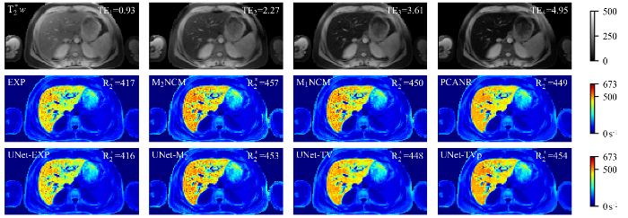
图7
一例中度铁沉积肝脏临床测试数据应用不同方法重建得到的$R^{*}_{2}$参数图像. 第一行显示了不同TE采集的$T^{*}_{2}$加权图像(TE1 = 0.93 ms,TE2 = 2.27 ms,TE3 = 3.61 ms,TE4 = 4.95 ms).肝实质内的平均$R^{*}_{2}$值(s-1)标于$R^{*}_{2}$参数图像的右上角. 图片右边色条颜色由蓝到红代表着$R^{*}_{2}$值从小到大的变化
Fig. 7
$R^{*}_{2}$ maps estimated by different reconstruction methods for one representative clinical testing data, which has moderate hepatic iron overload. First row: $T^{*}_{2}$-weighted images (TE1 = 0.93 ms, TE2 = 2.27 ms, TE3 = 3.61 ms, TE4 = 4.95 ms). The mean $R^{*}_{2}$ value (s-1) in liver parenchyma (excluding vasculatures) is shown in the top right corner of each $R^{*}_{2}$ map. The change of color in the color bar on the right side of the figure from blue to red represents the $R^{*}_{2}$ value from small to large
图8
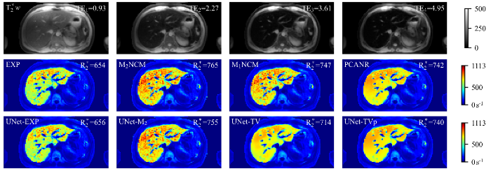
图8
一例重度铁沉积肝脏临床测试数据应用不同方法重建得到的$R^{*}_{2}$参数图像. 第一行显示了不同TE采集的$T^{*}_{2}$加权图像(TE1 = 0.93 ms,TE2 = 2.27 ms,TE3 = 3.61 ms,TE4 = 4.95 ms).肝实质内的平均$R^{*}_{2}$值(s-1)标于$R^{*}_{2}$参数图像的右上角. 图片右边色条颜色由蓝到红代表着$R^{*}_{2}$值从小到大的变化
Fig. 8
$R^{*}_{2}$ maps estimated by different reconstruction methods for one representative clinical testing data, which has severe hepatic iron overload. First row: $T^{*}_{2}$-weighted images (TE1 = 0.93 ms, TE2 = 2.27 ms, TE3 = 3.61 ms, TE4 = 4.95 ms). The mean $R^{*}_{2}$ value (s-1) in liver parenchyma (excluding vasculatures) is shown in the top right corner of each $R^{*}_{2}$ map. The change of color in the color bar on the right side of the figure from blue to red represents the $R^{*}_{2}$ value from small to large
3 讨论
本文提出了一种模型引导的自监督深度学习网络UNet-TVp用于铁沉积肝脏的$R_{2}^{*}$参数图像重建方法,利用一种噪声校正模型和一种改进的TV模型构建损失函数引导卷积神经网络的训练,使得网络只需要临床采集到的$T_{2}^{*}$加权图像进行训练,而不需要真实的或者高质量的$R_{2}^{*}$参数图像作为标签. 本文提出的方法能够很好地校正噪声引起的$R_{2}^{*}$估计偏差,同时抑制$R_{2}^{*}$参数图像中的噪声.
本文对提出的方法在仿真肝脏数据和临床肝脏数据上进行了评估. 肝脏$T_{2}^{*}$加权图像的噪声是一种非高斯分布的噪声,如果仅仅使用简单的单指数物理衰减模型进行拟合计算会引起$R_{2}^{*}$参数估计的偏差,如EXP和UNet-EXP的结果所示. 根据噪声的分布构建拟合模型能够有效的校正噪声引起的偏差,如M2NCM、M1NCM和UNet-M2的结果所示. 但是,逐像素点的拟合依旧会导致重建的$R_{2}^{*}$参数图像中存在噪声. 利用邻域相似性信息(如PCANR)或者参数图像的空间均匀的先验信息(如UNet-TV和UNet-TVp)对重建图像进行约束能够很好地抑制噪声的影响. UNet-TV在$R_{2}^{*}$值较大时重建得到的参数图像会损失一定的对比度,造成$R_{2}^{*}$的低估,而使用改进后的TV模型能够有效地保持参数图像的对比度,更准确地估计$R_{2}^{*}$参数值.
与当前最优的肝脏$R_{2}^{*}$参数图像重建方法PCANR相比,本文提出的方法UNet-TVp在仿真肝脏数据集上取得了更好的定量结果;在临床数据集上定性和定量的比较也具有很好的一致性,这将有助于肝脏铁含量的精确测量. 在为临床医生提供准确的肝脏$R_{2}^{*}$参数图像的同时,本文提出的方法提升了$R_{2}^{*}$参数图像的重建速度,极大地节省了临床应用过程中数据后处理的时间. 对于大小为64×128的二维肝脏数据,PCANR重建一副$R_{2}^{*}$参数图像的时间大约为20 s,而UNet-TVp在1 s之内就能重建出对应的$R_{2}^{*}$参数图像,这十分有利于临床的推广应用. 此外,一般的监督学习策略所需的真实参数图像或者高质量的参数图像在临床上通常是难以获得的,本文提出的方法提供了一种自监督学习框架,仅需要临床采集得到的带噪声的加权图像进行训练. 通过对噪声校正模型进行修改,本文提出的方法可以推广到其他参数图像的重建,例如T1、T2和DWI参数.
本研究也存在一定的局限性和不足. 本文提出的方法使用的卷积神经网络是基于常用的U-Net网络构建得到的,使用其他更为新颖先进的网络结构[23]可能会进一步提升方法的性能,或者利用3D网络[24]还可以将算法扩展到3D参数图像重建中. 网络训练时更好的阈值参数a和权重参数λ的组合可能会进一步提升UNet-TVp的性能,未来需要对参数的设置进行更加全面的研究. 当前实验仅对基于TV和改进的TV模型进行了研究,基于其它形式的降噪模型(例如,局部低秩模型[25]、稀疏模型[26]、RED模型[27])来构建损失函数可能会进一步提高算法的表现. 尽管使用了数据扩增技术,但用于网络训练的数据量是相对较少的,更多的训练数据有利于方法性能的提升. 在并行成像中,图像中的噪声水平依赖于空间位置,本文提出的方法当前只适用于噪声水平空间不变的情况,未来通过估计空间变化的噪声水平[28]可以进一步扩展本方法. 此外,本文使用的是临床容易获得的幅值图像作为网络的输入,未来应用复数图像来进行参数图像重建[29]可能会进一步提升重建的表现. 本研究当前着重于方法学研究,重点阐述了模型的构建过程和方法的可行性,并且在临床数据上验证了$R_{2}^{*}$估计的准确性. 为了进一步将其推广到临床肝脏铁沉积评估,我们未来将对本方法进行更加全面的临床评估验证,包括应用更多的临床数据,与有创的肝脏穿刺活检结果进行对比评估,进一步验证其肝脏铁含量测量的准确性.
4 结论
本文提出了一种用于铁沉积肝脏$R_{2}^{*}$参数图像重建的深度学习网络UNet-TVp,该网络通过噪声校正模型和改进的TV模型的引导,仅使用临床采集得到的肝脏$T_{2}^{*}$加权图像即可进行自监督训练. 该方法能够很好地抑制噪声对参数图像的影响,快速准确地重建得到铁沉积肝脏$R_{2}^{*}$参数图像. 另外,该方法可进一步推广应用到其他参数图像的重建任务中,例如T1、T2和DWI参数.
利益冲突
无
参考文献
Liver iron quantification with MR imaging: A primer for radiologists
[J].
DOI:10.1148/rg.2018170079
PMID:29528818
[本文引用: 1]

Iron overload is a systemic disorder and is either primary (genetic) or secondary (exogenous iron administration). Primary iron overload is most commonly associated with hereditary hemochromatosis and secondary iron overload with ineffective erythropoiesis (predominantly caused by β-thalassemia major and sickle cell disease) that requires long-term transfusion therapy, leading to transfusional hemosiderosis. Iron overload may lead to liver cirrhosis and hepatocellular carcinoma, in addition to cardiac and endocrine complications. The liver is one of the main iron storage organs and the first to show iron overload. Therefore, detection and quantification of liver iron overload are critical to initiate treatment and prevent complications. Liver biopsy was the historical reference standard for detection and quantification of liver iron content. Magnetic resonance (MR) imaging is now commonly used for liver iron quantification, including assessment of distribution, detection, grading, and monitoring of treatment response in iron overload. Several MR imaging techniques have been developed for iron quantification, each with advantages and limitations. The liver-to-muscle signal intensity ratio technique is simple and widely available; however, it assumes that the reference tissue is normal. Transverse magnetization (also known as R2) relaxometry is validated but is prone to respiratory motion artifacts due to a long acquisition time, is presently available only for 1.5-T imaging, and requires additional cost and delay for off-line analysis. The R2* technique has fast acquisition time, demonstrates a wide range of liver iron content, and is available for 1.5-T and 3.0-T imaging but requires additional postprocessing software. Quantitative susceptibility mapping has the highest sensitivity for detecting iron deposition; however, it is still investigational, and the correlation with liver iron content is not yet established. RSNA, 2018.
MRI R2 and R2* mapping accurately estimates hepatic iron concentration in transfusion-dependent thalassemia and sickle cell disease patients
[J].
DOI:10.1182/blood-2004-10-3982
URL
[本文引用: 1]
Measurements of hepatic iron concentration (HIC) are important predictors of transfusional iron burden and long-term outcome in patients with transfusion-dependent anemias. The goal of this work was to develop a readily available, noninvasive method for clinical HIC measurement. The relaxation rates R2 (1/T2) and R2* (1/T2*) measured by magnetic resonance imaging (MRI) have different advantages for HIC estimation. This article compares noninvasive iron estimates using both optimized R2 and R2* methods in 102 patients with iron overload and 13 controls. In the iron-overloaded group, 22 patients had concurrent liver biopsy. R2 and R2* correlated closely with HIC (r2 ≥.95) for HICs between 1.33 and 32.9 mg/g, but R2 had a curvilinear relationship to HIC. Of importance, the R2 calibration curve was similar to the curve generated by other researchers, despite significant differences in technique and instrumentation. Combined R2 and R2* measurements did not yield more accurate results than either alone. Both R2 and R2* can accurately measure hepatic iron concentration throughout the clinically relevant range of HIC with appropriate MRI acquisition techniques. (Blood. 2005;106:1460-1465)
MRI-T2* technique in quantitative analysis of myocardium, liver and pancreas iron deposition in β-thalassemia major and the correlations with glucose metabolism
[J].
MRI-T2*技术定量分析β-重型地中海贫血心脏、肝脏、胰腺铁沉积及其与糖代谢的相关性
[J].
Study on R2* combined with T1-mapping to evaluate iron overload in liver
[J].
磁共振R2*联合T1-mapping对肝脏铁过载评估的研究
[J].
Fast approximation to pixelwise relaxivity maps: Validation in iron overloaded subjects
[J].
DOI:10.1016/j.mri.2013.05.005
PMID:23773621
[本文引用: 1]
Liver iron quantification by MRI has become routine. Pixelwise (PW) fitting to the iron-mediated signal decay has some advantages but is slower and more vulnerable to noise than region-based techniques. We present a fast, pseudo-pixelwise mapping (PPWM) algorithm.The PPWM algorithm divides the entire liver into non-contiguous groups of pixels sorted by rapid relative relaxivity estimates. Pixels within each group of like-relaxivity were binned and fit using a Levenberg-Marquadt algorithm.The developed algorithm worked about 30 times faster than the traditional PW approach and generated R2* maps qualitatively and quantitatively similar. No systematic difference was observed in median R2* values with a coefficient of variability (CoV) of 2.4%. Intra-observer and inter-observer errors were also under 2.5%. Small systematic differences were observed in the right tail of the R2* distribution resulting in slightly lower mean R2* values (CoV of 4.2%) and moderately lower SD of R2* values for the PPWM algorithm. Moreover, the PPWM provided the best accuracy, giving a lower error of R2* estimates.The PPWM yielded comparable reproducibility and higher accuracy than the TPWM. The method is suitable for relaxivity maps in other organs and applications.Copyright © 2013 Elsevier Inc. All rights reserved.
Signal-to-noise measurements in magnitude images from NMR phased arrays
[J].A method is proposed to estimate signal-to-noise ratio (SNR) values in phased array magnitude images, based on a region-of-interest (ROI) analysis. It is shown that the SNR can be found by correcting the measured signal intensity for the noise bias effects and by evaluating the noise variance as the mean square value of all the pixel intensities in a chosen background ROI, divided by twice the number of receivers used. Estimated SNR values are shown to vary spatially within a bound of 20% with respect to the true SNR values as a result of noise correlations between receivers.
Improved MRI R2* relaxometry of iron-loaded liver with noise correction
[J].DOI:10.1002/mrm.v70.6 URL [本文引用: 4]
Improved liver R2* mapping by pixel-wise curve fitting with adaptive neighborhood regularization
[J].DOI:10.1002/mrm.v80.2 URL [本文引用: 4]
Rapid MR relaxometry using deep learning: An overview of current techniques and emerging trends
[J].DOI:10.1002/nbm.v35.4 URL [本文引用: 1]
U-net: Convolutional networks for biomedical image segmentation
[C]//
MANTIS: Model-augmented neural network with incoherent k-space sampling for efficient MR parameter mapping
[J].
DOI:10.1002/mrm.27707
PMID:30860285
[本文引用: 1]
To develop and evaluate a novel deep learning-based image reconstruction approach called MANTIS (Model-Augmented Neural neTwork with Incoherent k-space Sampling) for efficient MR parameter mapping.MANTIS combines end-to-end convolutional neural network (CNN) mapping, incoherent k-space undersampling, and a physical model as a synergistic framework. The CNN mapping directly converts a series of undersampled images straight into MR parameter maps using supervised training. Signal model fidelity is enforced by adding a pathway between the undersampled k-space and estimated parameter maps to ensure that the parameter maps produced synthesized k-space consistent with the acquired undersampling measurements. The MANTIS framework was evaluated on the T mapping of the knee at different acceleration rates and was compared with 2 other CNN mapping methods and conventional sparsity-based iterative reconstruction approaches. Global quantitative assessment and regional T analysis for the cartilage and meniscus were performed to demonstrate the reconstruction performance of MANTIS.MANTIS achieved high-quality T mapping at both moderate (R = 5) and high (R = 8) acceleration rates. Compared to conventional reconstruction approaches that exploited image sparsity, MANTIS yielded lower errors (normalized root mean square error of 6.1% for R = 5 and 7.1% for R = 8) and higher similarity (structural similarity index of 86.2% at R = 5 and 82.1% at R = 8) to the reference in the T estimation. MANTIS also achieved superior performance compared to direct CNN mapping and a 2-step CNN method.The MANTIS framework, with a combination of end-to-end CNN mapping, signal model-augmented data consistency, and incoherent k-space sampling, is a promising approach for efficient and robust estimation of quantitative MR parameters.© 2019 International Society for Magnetic Resonance in Medicine.
Magnetic resonance parameter mapping using model-guided self-supervised deep learning
[J].
DOI:10.1002/mrm.28659
PMID:33464652
[本文引用: 2]
To develop a model-guided self-supervised deep learning MRI reconstruction framework called reference-free latent map extraction (RELAX) for rapid quantitative MR parameter mapping.Two physical models are incorporated for network training in RELAX, including the inherent MR imaging model and a quantitative model that is used to fit parameters in quantitative MRI. By enforcing these physical model constraints, RELAX eliminates the need for full sampled reference data sets that are required in standard supervised learning. Meanwhile, RELAX also enables direct reconstruction of corresponding MR parameter maps from undersampled k-space. Generic sparsity constraints used in conventional iterative reconstruction, such as the total variation constraint, can be additionally included in the RELAX framework to improve reconstruction quality. The performance of RELAX was tested for accelerated T and T mapping in both simulated and actually acquired MRI data sets and was compared with supervised learning and conventional constrained reconstruction for suppressing noise and/or undersampling-induced artifacts.In the simulated data sets, RELAX generated good T /T maps in the presence of noise and/or undersampling artifacts, comparable to artifact/noise-free ground truth. The inclusion of a spatial total variation constraint helps improve image quality. For the in vivo T /T mapping data sets, RELAX achieved superior reconstruction quality compared with conventional iterative reconstruction, and similar reconstruction performance to supervised deep learning reconstruction.This work has demonstrated the initial feasibility of rapid quantitative MR parameter mapping based on self-supervised deep learning. The RELAX framework may also be further extended to other quantitative MRI applications by incorporating corresponding quantitative imaging models.© 2021 International Society for Magnetic Resonance in Medicine.
Rudin-Osher-Fatemi total variation denoising using split bregman
[J].DOI:10.5201/ipol URL [本文引用: 1]
Image denoising via anisotropic total-variation-based method
[J].
各向异性全变分图像去噪算法
[J].
Sparse MRI: The application of compressed sensing for rapid MR imaging
[J].
DOI:10.1002/mrm.21391
PMID:17969013
[本文引用: 1]
The sparsity which is implicit in MR images is exploited to significantly undersample k-space. Some MR images such as angiograms are already sparse in the pixel representation; other, more complicated images have a sparse representation in some transform domain-for example, in terms of spatial finite-differences or their wavelet coefficients. According to the recently developed mathematical theory of compressed-sensing, images with a sparse representation can be recovered from randomly undersampled k-space data, provided an appropriate nonlinear recovery scheme is used. Intuitively, artifacts due to random undersampling add as noise-like interference. In the sparse transform domain the significant coefficients stand out above the interference. A nonlinear thresholding scheme can recover the sparse coefficients, effectively recovering the image itself. In this article, practical incoherent undersampling schemes are developed and analyzed by means of their aliasing interference. Incoherence is introduced by pseudo-random variable-density undersampling of phase-encodes. The reconstruction is performed by minimizing the l(1) norm of a transformed image, subject to data fidelity constraints. Examples demonstrate improved spatial resolution and accelerated acquisition for multislice fast spin-echo brain imaging and 3D contrast enhanced angiography.(c) 2007 Wiley-Liss, Inc.
Image restoration using total variation regularized deep image prior
[C]//
Edge-preserving and scale-dependent properties of total variation regularization
[J].DOI:10.1088/0266-5611/19/6/059 URL [本文引用: 1]
A first-order image restoration model that promotes image contrast preservation
[J].DOI:10.1007/s10915-021-01519-7 [本文引用: 2]
Delving deep into rectifiers: Surpassing human-level performance on ImageNet classification
[C]//
Compressed sensing: From research to clinical practice with deep neural networks: shortening scan times for magnetic resonance imaging
[J].
Image quality assessment: From error visibility to structural similarity
[J].DOI:10.1109/TIP.2003.819861 URL [本文引用: 1]
scikit-image: image processing in Python
[J].DOI:10.7717/peerj.453 URL [本文引用: 1]
A deep recursive cascaded convolutional network for parallel MRI
[J].
基于深度递归级联卷积神经网络的并行磁共振成像方法
[J].
Automatic segmentation of knee joint synovial magnetic resonance images based on 3D VNetTrans
[J].
基于3D VNetTrans的膝关节滑膜磁共振图像自动分割
[J].
Accelerating parameter mapping with a locally low rank constraint
[J].
DOI:10.1002/mrm.25161
PMID:24500817
[本文引用: 1]
To accelerate MR parameter mapping using a locally low rank (LLR) constraint, and the combination of parallel imaging and the LLR constraint.An LLR method is developed for MR parameter mapping and compared with a globally low rank method in a multiecho spin-echo T2 mapping experiment. For acquisition with coil arrays, a combined LLR and parallel imaging method is proposed. The proposed method is evaluated in a variable flip angle T1 mapping experiment and compared with the LLR method and parallel imaging alone.In the multiecho spin-echo T2 mapping experiment, the LLR method is more accurate than the globally low rank method for acceleration factors 2 and 3, especially for tissues with high T2 values. Variable flip angle T1 mapping is achieved by acquiring datasets with 10 flip angles, each dataset accelerated by a factor of 6, and reconstructed by the proposed method with a small normalized root mean square error of 0.025.The LLR method is likely superior to the globally low rank method for MR parameter mapping. The proposed combined LLR and parallel imaging method has better performance than the two methods alone, especially with highly accelerated acquisition.© 2014 Wiley Periodicals, Inc.
Accelerated MR parameter mapping with low-rank and sparsity constraints
[J].
DOI:10.1002/mrm.25421
PMID:25163720
[本文引用: 1]
To enable accurate magnetic resonance (MR) parameter mapping with accelerated data acquisition, utilizing recent advances in constrained imaging with sparse sampling.A new constrained reconstruction method based on low-rank and sparsity constraints is proposed to accelerate MR parameter mapping. More specifically, the proposed method simultaneously imposes low-rank and joint sparse structures on contrast-weighted image sequences within a unified mathematical formulation. With a pre-estimated subspace, this formulation results in a convex optimization problem, which is solved using an efficient numerical algorithm based on the alternating direction method of multipliers.To evaluate the performance of the proposed method, two application examples were considered: (i) T2 mapping of the human brain and (ii) T1 mapping of the rat brain. For each application, the proposed method was evaluated at both moderate and high acceleration levels. Additionally, the proposed method was compared with two state-of-the-art methods that only use a single low-rank or joint sparsity constraint. The results demonstrate that the proposed method can achieve accurate parameter estimation with both moderately and highly undersampled data. Although all methods performed fairly well with moderately undersampled data, the proposed method achieved much better performance (e.g., more accurate parameter values) than the other two methods with highly undersampled data.Simultaneously imposing low-rank and sparsity constraints can effectively improve the accuracy of fast MR parameter mapping with sparse sampling.© 2014 Wiley Periodicals, Inc.
The little engine that could: Regularization by Denoising (RED)
[J].DOI:10.1137/16M1102884 URL [本文引用: 1]
Robust estimation of spatially variable noise fields
[J].
DOI:10.1002/mrm.22013
PMID:19526510
[本文引用: 1]
Consideration of spatially variable noise fields is becoming increasingly necessary in MRI given recent innovations in artifact identification and statistically driven image processing. Fast imaging methods enable study of difficult anatomical targets and improve image quality but also increase the spatial variability in the noise field. Traditional analysis techniques have either assumed that the noise is constant across the field of view (or region of interest) or have relied on separate MRI acquisitions to measure the noise field. These methods are either inappropriate for many modern scanning protocols or are overly time-consuming for already lengthy scanning sessions. We propose a new, general framework for estimating spatially variable noise fields from related, but independent MR scans that we call noise field equivalent scans. These heuristic analyses enable robust noise field estimation in the presence of artifacts. Generalization of noise estimators based on uniform regions, difference images, and maximum likelihood are presented and compared with the estimators derived from the proposed framework. Simulations of diffusion tensor imaging and T(2)-relaxometry demonstrate a 10-fold reduction in mean squared error in noise field estimation, and these improvements are shown to be robust to artifact contamination. In vivo studies show that spatially variable noise fields can be readily estimated with typical data acquired at 1.5T.(c) 2009 Wiley-Liss, Inc.
Practical guide to quantification of hepatic iron with MRI
[J].
DOI:10.1007/s00330-019-06380-9
PMID:31392478
[本文引用: 1]
Our intention is to demystify the MR quantification of hepatic iron (i.e., the liver iron concentration) and give you a step-by-step approach by answering the most pertinent questions. The following article should be more of a manual or guide for every radiologist than a classic review article, which just summarizes the literature. Furthermore, we provide important background information for professional communication with clinicians. The information regarding the physical background is reduced to a minimum. After reading this article, you should be able to perform adequate MR measurements of the LIC with 1.5-T or 3.0-T scanners. KEY POINTS: • MRI is widely accepted as the primary approach to non-invasively determine liver iron concentration (LIC). • This article is a guide for every radiologist to perform adequate MR measurements of the LIC. • When using R2* relaxometry, some points have to be considered to obtain correct measurements-all explained in this article.
